Laplacian

We are interested in this section in the conforming finite element approximation of the following problem:

Laplacian problem

Look for $u$ such that

$\left\{\begin{split} -\Delta u &= f \text{ in } \Omega\\ u &= g \text{ on } \partial \Omega_D\\ \frac{\partial u}{\partial n} &=h \text{ on } \partial \Omega_N\\ \frac{\partial u}{\partial n} + u &=l \text{ on } \partial \Omega_R \end{split}\right.$

$\partial \Omega_D$ ,

$\partial \Omega_N$ and

$\partial \Omega_R$ can be empty sets. In the case

$\partial \Omega_D =\partial \Omega_R = \emptyset$ , then the solution is known up to a constant.

Hereafter, we note

$\Gamma_D=\partial \Omega_D$ ,

$\Gamma_N=\partial \Omega_N$ and

$\Gamma_R=\partial \Omega_R$ .

In the implementation presented later, $\partial \Omega_D =\partial \Omega_N = \partial \Omega_R = \emptyset$ , then we set Dirichlet boundary conditions all over the boundary. The problem then reads like a standard laplacian with inhomogeneous Dirichlet boundary conditions:

Laplacian Problem with inhomogeneous Dirichlet conditions

Look for $u$ such that

Inhomogeneous Dirichlet Laplacian problem

$-\Delta u = f\ \text{ in } \Omega,\quad u = g \text{ on } \partial \Omega$

1. Variational formulation

We assume that $f, h, l \in L^2(\Omega)$ . The weak formulation of the problem then reads:

Laplacian problem variational formulation

Look for $u \in H^1_{g,\Gamma_D}(\Omega)$ such that

Variational formulation

$\displaystyle\int_\Omega \nabla u \cdot \nabla v +\int_{\Gamma_R} u v = \displaystyle \int_\Omega f\ v+ \int_{\Gamma_N} g\ v + \int_{\Gamma_R} l\ v,\quad \forall v \in H^1_{0,\Gamma_D}(\Omega)$

2. Conforming Approximation

We now turn to the finite element approximation using Lagrange finite element. We assume $\Omega$ to be a segment in 1D, a polygon in 2D or a polyhedron in 3D. We denote $V_\delta \subset H^1(\Omega)$ an approximation space such that $V_{g,\delta} \equiv P^k_{c,\delta}\cap H^1_{g,\Gamma_D}(\Omega)$ .

The weak formulation reads:

Laplacian problem weak formulation

Look for $u_\delta \in V_\delta$ such that

$\displaystyle\int_{\Omega_\delta} \nabla u_{\delta} \cdot \nabla v_\delta +\int_{\Gamma_{R,\delta}} u_\delta\ v_\delta = \displaystyle \int_{\Omega_\delta} f\ v_\delta+ \int_{\Gamma_{N,\delta}} g\ v_\delta + \int_{\Gamma_{R,\delta}} l\ v_\delta,\quad \forall v_\delta \in V_{0,\delta}$

from now on, we omit

$\delta$ to lighten the notations. Be careful that it appears both the geometrical and approximation level.

3. Feel++ Implementation

In Feel++, $V_{g,\delta}$ is not built but rather $P^k_{c,\delta}$ .

The Dirichlet boundary conditions can be treated using different techniques and we use from now on the elimination technique.

We start with the mesh

    auto mesh = loadMesh(_mesh=new Mesh<Simplex<FEELPP_DIM,1>>);cpp

the keyword auto enables type inference, for more details see Wikipedia C++11 page.

    auto Vh = Pch<2>( mesh ); (1)
    auto u = Vh->element("u"); (2)
    auto mu = expr(soption(_name="functions.mu")); // diffusion term (3)
    auto f = expr( soption(_name="functions.f"), "f" ); (4)
    auto r_1 = expr( soption(_name="functions.a"), "a" ); // Robin left hand side expression (5)
    auto r_2 = expr( soption(_name="functions.b"), "b" ); // Robin right hand side expression (6)
    auto n = expr( soption(_name="functions.c"), "c" ); // Neumann expression (7)
    auto solution = expr( checker().solution(), "solution" ); (8)
    auto g = checker().check()?solution:expr( soption(_name="functions.g"), "g" ); (9)
    auto v = Vh->element( g, "g" ); (3)cpp

Next we define

1	the discrete space `Vh=Pch<k>(mesh)` $\equiv P^k_{c,h}$ ,
2	an element `u` of `Vh`
3	an expression `mu` that is used as the diffusion coefficient
4	an expression `f` that is used for the right hand-side term in the equation
5	an expression `r_1` that is used for the first term in the Robin boundary condition
6	an expression `r_2` that is used for the first term in the Robin boundary condition
7	an expression `n` that is used to define the Neumann boundary condition
8	an expression `solution` that is used to define the exact solution if there is one
9	an expression `g` that is used to define the Dirichlet boundary condition.

at the following line

    auto v = Vh->element( g, "g" ); (3)cpp

v is set to the expression g, which means more precisely that v is the interpolant of g in Vh, i.e we write $v=\Pi^k_{c,\delta} g$ with $v \in P^k_{c,\delta}$ .

the variational formulation is implemented below, we define the bilinear form a and linear form l and we set strongly the Dirichlet boundary conditions with the keyword on using elimination. If we don’t find Dirichlet, Neumann or Robin in the list of physical markers in the mesh data structure then we impose Dirichlet boundary conditions all over the boundary.

    tic();
    auto l = form1( _test=Vh );
    l = integrate(_range=elements(mesh),
                  _expr=f*id(v));
    l+=integrate(_range=markedfaces(mesh,"Robin"), _expr=r_2*id(v));
    l+=integrate(_range=markedfaces(mesh,"Neumann"), _expr=n*id(v));
    toc("l");

    tic();
    auto a = form2( _trial=Vh, _test=Vh);
    tic();
    a = integrate(_range=elements(mesh),
                  _expr=mu*inner(gradt(u),grad(v)) );
    toc("a");
    a+=integrate(_range=markedfaces(mesh,"Robin"), _expr=r_1*idt(u)*id(v));
    a+=on(_range=markedfaces(mesh,"Dirichlet"), _rhs=l, _element=u, _expr=g );
    //! if no markers Robin Neumann or Dirichlet are present in the mesh then
    //! impose Dirichlet boundary conditions over the entire boundary
    if ( !mesh->hasAnyMarker({"Robin", "Neumann","Dirichlet"}) )
        a+=on(_range=boundaryfaces(mesh), _rhs=l, _element=u, _expr=g );
    toc("a");cpp

We have the following correspondence:

Element sets Domain

elements(mesh)

$\Omega$

boundaryfaces(mesh)

$\partial \Omega$

markedfaces(mesh,"Dirichlet")

$\Gamma_D$

markedfaces(mesh,"Neumann")

$\Gamma_R$

markedfaces(mesh,"Robin")

$\Gamma_R$

More details can be found in Mathematical keywords of Feel++ and the Mesh reference.

next we solve the algebraic problem

Listing: solve algebraic system

    tic();
    //! solve the linear system, find u s.t. a(u,v)=l(v) for all v
    if ( !boption( "no-solve" ) )
        a.solve(_rhs=l,_solution=u);
    toc("a.solve");cpp

next we compute the $L^2$ norm of $u_\delta-g$ , it could serve as an $L^2$ error if $g$ was manufactured to be the exact solution of the Laplacian problem.

    // compute l2 and h1 norm of u-u_h where u=solution
    auto norms = [=]( std::string const& solution ) ->std::map<std::string,double>
        {
            tic();
            double l2 = normL2(_range=elements(mesh), _expr=idv(u)-expr(solution) );
            toc("L2 error norm");
            tic();
            double h1 = normH1(_range=elements(mesh), _expr=idv(u)-expr(solution), _grad_expr=gradv(u)-grad<2>(expr(solution)) );
            toc("H1 error norm");
            return { { "L2", l2 }, {  "H1", h1 } };
        };

    int status = checker().runOnce( norms, rate::hp( mesh->hMax(), Vh->fe()->order() ) );cpp

and finally we export the results, by default it is in the ensight gold format and the files can be read with Paraview and Ensight. We save both $u$ and $g$ .

Listing: export Laplacian results

    tic();
    auto e = exporter( _mesh=mesh );
    e->addRegions();
    e->add( "uh", u );
    if ( checker().check() )
    {
        v.on(_range=elements(mesh), _expr=solution );
        e->add( "solution", v );
    }
    e->save();
    toc("Exporter");cpp

The full listing is available below

Listing: feelpp_qs_laplacian_2d and feelpp_qs_laplacian_3d

#include <feel/feel.hpp>

int main(int argc, char**argv )
{
    using namespace Feel;
    using Feel::cout;
    po::options_description laplacianoptions( "Laplacian options" );
    laplacianoptions.add_options()
        ( "no-solve", po::value<bool>()->default_value( false ), "No solve" )
        ;

    Environment env( _argc=argc, _argv=argv,
                   _desc=laplacianoptions,
                   _about=about(_name="qs_laplacian",
                                _author="Feel++ Consortium",
                                _email="feelpp-devel@feelpp.org"));

    tic();
    auto mesh = loadMesh(_mesh=new Mesh<Simplex<FEELPP_DIM,1>>);
    toc("loadMesh");

    tic();
    auto Vh = Pch<2>( mesh ); (1)
    auto u = Vh->element("u"); (2)
    auto mu = expr(soption(_name="functions.mu")); // diffusion term (3)
    auto f = expr( soption(_name="functions.f"), "f" ); (4)
    auto r_1 = expr( soption(_name="functions.a"), "a" ); // Robin left hand side expression (5)
    auto r_2 = expr( soption(_name="functions.b"), "b" ); // Robin right hand side expression (6)
    auto n = expr( soption(_name="functions.c"), "c" ); // Neumann expression (7)
    auto solution = expr( checker().solution(), "solution" ); (8)
    auto g = checker().check()?solution:expr( soption(_name="functions.g"), "g" ); (9)
    auto v = Vh->element( g, "g" ); (3)
    toc("Vh");

    tic();
    auto l = form1( _test=Vh );
    l = integrate(_range=elements(mesh),
                  _expr=f*id(v));
    l+=integrate(_range=markedfaces(mesh,"Robin"), _expr=r_2*id(v));
    l+=integrate(_range=markedfaces(mesh,"Neumann"), _expr=n*id(v));
    toc("l");

    tic();
    auto a = form2( _trial=Vh, _test=Vh);
    tic();
    a = integrate(_range=elements(mesh),
                  _expr=mu*inner(gradt(u),grad(v)) );
    toc("a");
    a+=integrate(_range=markedfaces(mesh,"Robin"), _expr=r_1*idt(u)*id(v));
    a+=on(_range=markedfaces(mesh,"Dirichlet"), _rhs=l, _element=u, _expr=g );
    //! if no markers Robin Neumann or Dirichlet are present in the mesh then
    //! impose Dirichlet boundary conditions over the entire boundary
    if ( !mesh->hasAnyMarker({"Robin", "Neumann","Dirichlet"}) )
        a+=on(_range=boundaryfaces(mesh), _rhs=l, _element=u, _expr=g );
    toc("a");

    tic();
    //! solve the linear system, find u s.t. a(u,v)=l(v) for all v
    if ( !boption( "no-solve" ) )
        a.solve(_rhs=l,_solution=u);
    toc("a.solve");

    tic();
    auto e = exporter( _mesh=mesh );
    e->addRegions();
    e->add( "uh", u );
    if ( checker().check() )
    {
        v.on(_range=elements(mesh), _expr=solution );
        e->add( "solution", v );
    }
    e->save();
    toc("Exporter");

    // compute l2 and h1 norm of u-u_h where u=solution
    auto norms = [=]( std::string const& solution ) ->std::map<std::string,double>
        {
            tic();
            double l2 = normL2(_range=elements(mesh), _expr=idv(u)-expr(solution) );
            toc("L2 error norm");
            tic();
            double h1 = normH1(_range=elements(mesh), _expr=idv(u)-expr(solution), _grad_expr=gradv(u)-grad<2>(expr(solution)) );
            toc("H1 error norm");
            return { { "L2", l2 }, {  "H1", h1 } };
        };

    int status = checker().runOnce( norms, rate::hp( mesh->hMax(), Vh->fe()->order() ) );

    // exit status = 0 means no error
    return !status;

}cpp

4. Test Cases

We are now ready to test this Laplacian Feel++ Implementation with 2D and 3D test cases.

The test cases are available in Docker in the directory (/usr/local/share/feelpp/testcases/quickstart/laplacian).

4.1. Circle

Circle is a 2D testcase where $\Omega \subset \RR^2$ is a disk whose boundary has been split such that $\partial \Omega=\partial \Omega_D \cup \partial \Omega_N \cup \partial \Omega_R$ .

In the following, we consider a manufactured solution $u=x^2+y^2$ and we would like to verify the a priori convergence finite element property.

This test case is tricky because the

$\partial \Omega$ is curved and

$\partial \Omega \neq \partial \Omega_h$ . Depending on the boundary condition type and in particular the definition of the normal, we may obtain the proper convergence rate or not.

We provide here the basic geometry used in Gmsh to describe $\Omega$ .

Description of the geometry in Gmsh

h=0.1;
Point(1) = {0, 0, 0, h};
Point(2) = {1, 0, 0, h};
Point(3) = {-1, 0, 0, h};
Point(4) = {0, 1, 0, h};
Point(5) = {0, -1, 0, h};
Circle(1) = {2, 1, 4};
Circle(2) = {4, 1, 3};
Circle(3) = {3, 1, 5};
Circle(5) = {5, 1, 2};
Line Loop(6) = {1, 2, 3, 5};
Plane Surface(7) = {6};cpp

The Circle curve has several sections (1,2,3,5) that will be used to define the different boundary conditions, Dirichlet, Neumann and Robin.

4.1.1. The case $\partial \Omega=\partial \Omega_D$

We start with Dirichlet conditions on $\partial \Omega$ which means that $\partial \Omega_N = \partial \Omega_R = \emptyset$ . To this end, we mark all boundary sections (1,2,3,5) as Dirichlet as shown in the Gmsh geo file below

Physical definition in Gmsh for

$\partial \Omega=\partial \Omega_D$ in circle-dirichlet.geo

Physical Line("Dirichlet") = {1, 2, 3, 5};
Physical Surface(8) = {7};cpp

The next step is to provide the proper conditions or expressions to Feel++ application feelpp_qs_laplacian_2d. They are described in the .cfg file.

Listing: expression section in the cfg file circle-dirichlet.cfg

[functions]
# Dirichlet
g=x^2+y^2:x:y
# right hand side
f=-4
# Robin left hand side
a=1
# Robin right hand side
b=2*(x*nx+y*ny)+x^2+y^2:x:y:nx:ny
# Neumann
c=2*(x*nx+y*ny):x:y:nx:ny
# mu: diffusion term (laplacian) (1)
mu=1ini

In the Dirichlet case, we do not have the issue mentioned above regarding the definition of the boundary and in particular the unit exterior normal to the boundary. We require only a point-wise evaluation of the condition on the boundary which are numerically exact.

We are now ready to run the application.

$ cd /usr/local/share/feelpp/testcases/quickstart/laplacian/circle
$ mpirun -np 4 feelpp_qs_laplacian_2d --config-file circle-dirichlet.cfgbash

The execution should look like this:

Reading /usr/local/share/feelpp/testcases/quickstart/laplacian/circle/circle-dirichlet.cfg...
[ Starting Feel++ ] application qs_laplacian version 0.104.0-alpha.40 date 2018-Apr-17
 . qs_laplacian files are stored in /feel/qs_laplacian/circle-dirichlet/np_1
 .. logfiles :/feel/qs_laplacian/circle-dirichlet/np_1/logs
[loadMesh] Loading mesh in format geo+msh: "/usr/local/share/feelpp/testcases/quickstart/laplacian/circle/circle-dirichlet.geo"
[loadMesh] Use default geo desc: /usr/local/share/feelpp/testcases/quickstart/laplacian/circle/circle-dirichlet.geo 0.1
[loadMesh] Time : 0.0689365s
[Vh] Time : 0.0120969s
[l] Time : 0.0180983s
 [a] Time : 0.0378079s
[a] Time : 0.0507547s
[a.solve] Time : 0.0267429s
 [Exporter] Time : 0.0319186s
 [L2 error norm] Time : 0.00716316s
 [H1 error norm] Time : 0.0263121s
Checker exact verification failed for ||u-u_h||_H1
 Computed error 1.39788e-14 (1)
 Tolerance 1e-15
Checker exact verification failed for ||u-u_h||_L2
 Computed error 1.54287e-15 (2)
 Tolerance 1e-15
[env] Time : 0.246247s
[ Stopping Feel++ ] application qs_laplacian execution time 0.246247ssh

1	provides the $H^1$ norm of the error with respect to the exact solution $x^2+y^2$
2	provides the $L^2$ norm of the error with respect to the exact solution $x^2+y^2$

The error norms reached machine precision, the solution is in the finite element space. It is due to the fact that (i) we used

$P^2$ finite elements, (ii) the solution is itself quadratic and (iii) we used Dirichlet boundary conditions which requires only point-wise evaluation of the solution on the curved boundary. The fact that the boundary is curved do not affect the numerical solution. It won’t be the case in the presence of Neumann and Robin conditions.

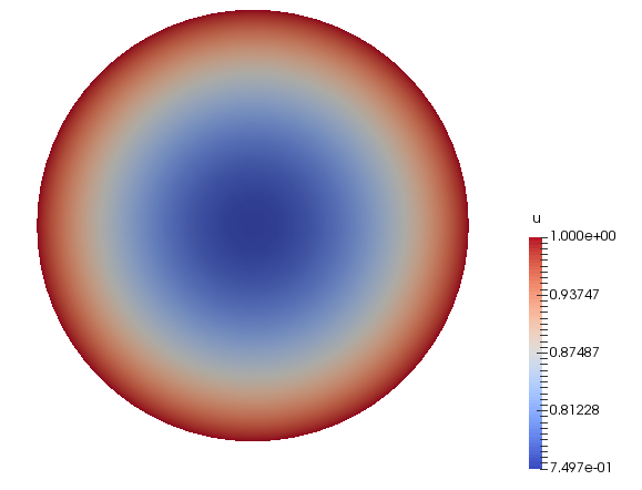
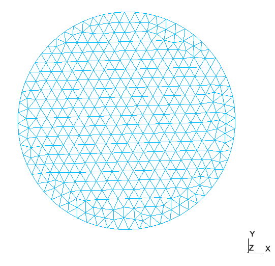
This gives us some data such as solution of our problem or the mesh used in the application which we can visualize using Paraview.

ucircle

meshCircle

Solution $u_\delta$

Mesh

4.1.2. The case $\partial \Omega=\partial \Omega_N$

We continue with Neumann conditions on $\partial \Omega$ which means that $\partial \Omega_D = \partial \Omega_R = \emptyset$ . To this end, we mark all boundary sections (1,2,3,5) as Neumann as shown in the Gmsh geo file below

Physical definition in Gmsh for

$\partial \Omega=\partial \Omega_N$ in circle-neumann.geo

Physical Line("Neumann") = {1, 2, 3, 5};
Physical Surface(8) = {7};cpp

The next step is to provide the proper conditions or expressions to Feel++ application feelpp_qs_laplacian_2d. They are described in the .cfg file.

Listing: expression section in the cfg file circle-neumann.cfg

[functions]
# dirichlet
g=x^2+y^2:x:y
# right hand side
f=-4
# robin
a=1
b=2*(x*nx+y*ny)+x^2+y^2:x:y:nx:ny
# neumann
c=2*(x*nx+y*ny):x:y:nx:ny
# mu: diffusion term (laplacian) (1)
mu=1ini

In the Neumann case, we do have the issue mentioned above regarding the definition of the boundary and in particular the unit exterior normal to the boundary. To remedy this problem, we compute the error with respect to the solution defined on $\Omega_h$ which is a polygon and not a circle. Hence the use of (nx,ny) which provide the normal components at the current point on the boundary.

We are now ready to run the application.

$ cd /usr/local/share/feelpp/testcases/quickstart/laplacian/circle
$ mpirun -np 4 feelpp_qs_laplacian_2d --config-file circle-neumann.cfgbash

The error norms reached machine precision, the solution is in the finite element space. It is due to the fact that (i) we used

This gives us some data such as solution of our problem or the mesh used in the application which we can visualize using Paraview. The solution is the same as in [fig:circle-1].

4.2. The case $\partial \Omega=\partial \Omega_D \cup \partial \Omega_N \cup \partial \Omega_R$

We finish with all boundary condition types on $\partial \Omega$ which means that $\partial \Omega_D$ $\partial \Omega_R$ and $\partial \Omega_N$ are non-empty sets. To this end, we mark all boundary sections (1,2) as Dirichlet, (3) as Neumann and (5) as Robin as shown in the Gmsh geo file below

Physical definition in Gmsh for all condition support in circle-all.geo

Physical Line("Dirichlet") = {1, 2};
Physical Line("Neumann") = {3};
Physical Line("Robin") = {5};
Physical Surface(8) = {7};cpp

The next step is to provide the proper conditions or expressions to Feel++ application feelpp_qs_laplacian_2d. They are described in the .cfg file.

Listing: expression section in the cfg file circle-all.cfg

[functions]
# dirichlet
g=x^2+y^2:x:y
# right hand side
f=-4
# robin
a=1
b=2*(x*nx+y*ny)+x^2+y^2:x:y:nx:ny
# neumann
c=2*(x*nx+y*ny):x:y:nx:ny
# mu: diffusion term (laplacian) (1)
mu=1ini

We are now ready to run the application.

$ cd /usr/local/share/feelpp/testcases/quickstart/laplacian/circle
$ mpirun -np 4 feelpp_qs_laplacian_2d --config-file circle-all.cfgbash

The error norms reached machine precision, the solution is in the finite element space. It is due to the fact that (i) we used

This gives us some data such as solution of our problem or the mesh used in the application which we can visualize using Paraview. The solution is the same as in [fig:circle-1].

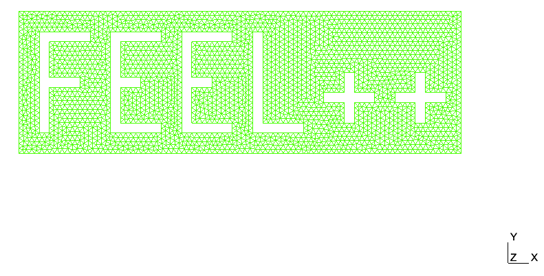
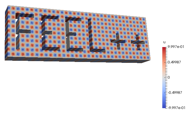
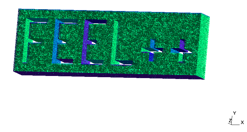
4.3. feelpp2d and feelpp3d

This testcase solves the Laplacian problem in $\Omega$ an quadrangle or hexadra containing the letters of Feel++

4.3.1. feelpp2d

After running the following command

cd Testcases/quickstart/feelpp2d
mpirun -np 4 /usr/local/bin/feelpp_qs_laplacian_2d --config-file feelpp2d.cfgbash

we obtain the result $u_\delta$ and also the mesh

image: laplacian/TestCases/Feelpp2d/ufeelpp2d.png[]

meshfeelpp2d

Solution $u_\delta$

Mesh

4.3.2. feelpp3d

We can launch this application with the current line

cd Testcases/quickstart/feelpp3d
mpirun -np 4 /usr/local/bin/feelpp_qs_laplacian_3d --config-file feelpp3d.cfgbash

When it’s finish, we can extract some informations

ufeelpp3d

meshfeelpp3d

Solution $u_\delta$

Mesh

Laplacian

1. Variational formulation

2. Conforming Approximation

3. Feel++ Implementation

4. Test Cases

4.1. Circle

4.1.1. The case ∂Ω=∂ΩD\partial \Omega=\partial \Omega_D

4.1.2. The case ∂Ω=∂ΩN\partial \Omega=\partial \Omega_N

4.2. The case ∂Ω=∂ΩD∪∂ΩN∪∂ΩR\partial \Omega=\partial \Omega_D \cup \partial \Omega_N \cup \partial \Omega_R

4.3. feelpp2d and feelpp3d

4.3.1. feelpp2d

4.3.2. feelpp3d

4.1.1. The case $\partial \Omega=\partial \Omega_D$

4.1.2. The case $\partial \Omega=\partial \Omega_N$

4.2. The case $\partial \Omega=\partial \Omega_D \cup \partial \Omega_N \cup \partial \Omega_R$