TP1

We consider the problem of designing a thermal fin to effectively remove heat from a surface. The two-dimensional fin, shown in Figure #fig:1[1], consists of a vertical central “post” and four horizontal “subfins”; the fin conducts heat from a prescribed uniform flux “source” at the root, \(\Gamma_{\mathrm{root}}\) , through the large-surface-area subfins to surrounding flowing air. The fin is characterized by a five-component parameter vector, or “input,” \(\mu_ = (\mu_1 , \mu_2, \ldots, \mu_5 )\),where \(\mu_i = k^i , i = 1, \ldots , 4\), and \(\mu_5 = \mathrm{Bi}\); \(\mu\) may take on any value in a specified design set \(D \subset \mathbb{R}^5\).

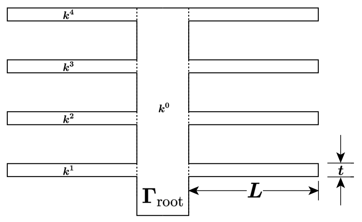
Here \(k^i\) is the thermal conductivity of the ith subfin (normalized relative to the post conductivity \(k^0 \equiv 1\)); and \(\mathrm{Bi}\) is the Biot number, a nondimensional heat transfer coefficient reflecting convective transport to the air at the fin surfaces (larger \(\mathrm{Bi}\) means better heat transfer). For example, suppose we choose a thermal fin with \(k^1 = 0.4, k^2 = 0.6, k^3 = 0.8, k^4 = 1.2\), and \(\mathrm{Bi} = 0.1\); for this particular configuration \(\mu = \{0.4, 0.6, 0.8, 1.2, 0.1\}\), which corresponds to a single point in the set of all possible configurations D (the parameter or design set). The post is of width unity and height four; the subfins are of fixed thickness \(t = 0.25\) and length \(L = 2.5\).

We are interested in the design of this thermal fin, and we thus need to look at certain outputs or cost-functionals of the temperature as a function of \(\mu\). We choose for our output \(T_{\mathrm{root}}\), the average steady-state temperature of the fin root normalized by the prescribed heat flux into the fin root. The particular output chosen relates directly to the cooling efficiency of the fin — lower values of \(T_{\mathrm{root}}\) imply better thermal performance. The steady–state temperature distribution within the fin, \(u(\mu)\), is governed by the elliptic partial differential equation

where \(\Delta\) is the Laplacian operator, and \(u_i\) refers to the restriction of \(u \text{ to } \Omega^i\) . Here \(\Omega^i\) is the region of the fin with conductivity \(k^i , i = 0,\ldots, 4: \Omega^0\) is thus the central post, and \(\Omega^i , i = 1,\ldots, 4\), corresponds to the four subfins. The entire fin domain is denoted \(\Omega (\bar{\Omega} = \cup_{i=0}^4 \bar{\Omega}^i )\); the boundary \(\Omega\) is denoted \(\Gamma\). We must also ensure continuity of temperature and heat flux at the conductivity– discontinuity interfaces \(\Gamma^i_{int} \equiv \partial\Omega^0 \cap \partial\Omega^i , i = 1,\ldots, 4\), where \(\partial\Omega^i\) denotes the boundary of \(\Omega^i\), we have on \(\Gamma^i_{int} i = 1,\ldots, 4\) :

here \(n^i\) is the outward normal on \(\partial\Omega^i\) . Finally, we introduce a Neumann flux boundary condition on the fin root

which models the heat source; and a Robin boundary condition

which models the convective heat losses. Here \(\Gamma^i_{ext}\) is that part of the boundary of \(\Omega^i\) exposed to the flowing fluid; note that \(\cup_{i=0}^4 \Gamma^i_{ext} = \Gamma\backslash\Gamma_{\mathrm{root}}\). The average temperature at the root, \(T_{\mathrm{root}} (\mu)\), can then be expressed as \(\ell^O(u(\mu))\), where

(recall \(\Gamma_{\mathrm{root}}\) is of length unity). Note that \(\ell(v) = \ell^O(v)\) for this problem.