Theory of Solid Mechanics

1. Notations and units

Notation

Quantity

Unit

$\boldsymbol{\eta}_s$

displacement

$m$

$\rho_s$

density

$kg.m^{-3}$

$\lambda_s$

first Lamé coefficients

$N.m^{-2}$

$\mu_s$

second Lamé coefficients

$N.m^{-2}$

$E_s$

Young modulus

$kg.m^{-1}.s^{-2}$

$\nu_s$

Poisson’s ratio

dimensionless

$\boldsymbol{F}_s$

deformation gradient

$\boldsymbol{\Sigma}_s$

second Piola-Kirchhoff tensor

$f_s^t$

body force

strain tensor $\boldsymbol{F}_s = \boldsymbol{I} + \nabla \boldsymbol{\eta}_s$
Cauchy-Green tensor $\boldsymbol{C}_s = \boldsymbol{F}_s^{T} \boldsymbol{F}_s$
Green-Lagrange tensor

$\begin{align} \boldsymbol{E}_s &= \frac{1}{2} \left( \boldsymbol{C}_s - \boldsymbol{I} \right) \\ &= \underbrace{\frac{1}{2} \left( \nabla \boldsymbol{\eta}_s + \left(\nabla \boldsymbol{\eta}_s\right)^{T} \right)}_{\boldsymbol{\epsilon}_s} + \underbrace{\frac{1}{2} \left(\left(\nabla \boldsymbol{\eta}_s\right)^{T} \nabla \boldsymbol{\eta}_s \right)}_{\boldsymbol{\gamma}_s} \end{align}$

2. Equations

Newton’s second law allows us to define the fundamental equation of solid mechanics, as follows

$\rho^*_{s} \frac{\partial^2 \boldsymbol{\eta}_s}{\partial t^2} - \nabla \cdot \left(\boldsymbol{F}_s \boldsymbol{\Sigma}_s\right) = \boldsymbol{f}^t_s$

2.1. Linear elasticity

$\begin{align} \boldsymbol{F}_s &= \text{Identity} \\ \boldsymbol{\Sigma}_s &=\lambda_s tr( \boldsymbol{\epsilon}_s)\boldsymbol{I} + 2\mu_s\boldsymbol{\epsilon}_s \end{align}$

2.2. Hyperelasticity

2.2.1. Saint-Venant-Kirchhoff

$\boldsymbol{\Sigma}_s=\lambda_s tr( \boldsymbol{E}_s)\boldsymbol{I} + 2\mu_s\boldsymbol{E}_s$

2.2.2. Neo-Hookean

$\boldsymbol{\Sigma}_s= \mu_s J^{-2/3}(\boldsymbol{I} - \frac{1}{3} \text{tr}(\boldsymbol{C}) \ \boldsymbol{C}^{-1})$

$\boldsymbol{\Sigma}_s^ = \boldsymbol{\Sigma}_s^\text{iso} + \boldsymbol{\Sigma}_s^\text{vol}$

Isochoric part : $\boldsymbol{\Sigma}_s^\text{iso}$

Table 1. Isochoric law
Name	$\mathcal{W}_S(J_s)$	$\boldsymbol{\Sigma}_s^{\text{iso}}$
Neo-Hookean		$\mu_s J^{-2/3}(\boldsymbol{I} - \frac{1}{3} \text{tr}(\boldsymbol{C}) \ \boldsymbol{C}^{-1})$

Volumetric part : $\boldsymbol{\Sigma}_s^\text{vol}$

Table 2. Volumetric law
Name	$\mathcal{W}_S(J_s)$	$\boldsymbol{\Sigma}_s^\text{vol}$
classic	$\frac{\kappa}{2} \left( J_s - 1 \right)^2$
simo1985	$\frac{\kappa}{2} \left( ln(J_s) \right)$

2.3. Axisymmetric reduced model

Here, we are interested in a 1D reduced model, named generalized string.

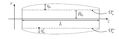
The axisymmetric form, which will interest us here, is a tube of length $L$ and radius $R_0$ . It is oriented following the $z$ axis and $r$ represents the radial axis. The reduced domain, named $\Omega_s^*$ is represented by the dotted line. So, the radial displacement $\eta_s$ is calculated in the domain $\Omega_s^*=\lbrack0,L\rbrack$ .

We introduce then $\Omega_s^{'*}$ , where we also need to estimate a radial displacement as before. The unique variance is this displacement direction.

Figure 1 : Geometry of the reduced model

The mathematical problem associated to this reduced model can be described as

$\rho^*_s h \frac{\partial^2 \eta_s}{\partial t^2} - k G_s h \frac{\partial^2 \eta_s}{\partial x^2} + \frac{E_s h}{1-\nu_s^2} \frac{\eta_s}{R_0^2} - \gamma_v \frac{\partial^3 \eta}{\partial x^2 \partial t} = f_s.$

where $\eta_s$ is the radial displacement that satisfies this equation, $k$ is the Timoshenko’s correction factor, and $\gamma_v$ is a viscoelasticity parameter. The material is defined by its density $\rho_s^*$ , its Young’s modulus $E_s$ , its Poisson’s ratio $\nu_s$ and its shear modulus $G_s$

In the end, we take $\eta_s=0\text{ on }\partial\Omega_s^*$ as a boundary condition, which will fix the wall to its extremities.