 .pdf
.pdf
Chapter 2 - Bounding Volume Hierarchy (BVH)
Chapter 2 provides a comprehensive overview of the Bounding Volume Hierarchy (BVH). In the introduction, the importance of Ray-Tracing is discussed and how BVH plays a crucial role in improving the speed and efficiency of the light transport simulation. The definition section elaborates on the concepts of Bounding Volumes, with detailed explanations on Axis-Aligned Bounding Boxes (AABBs) and Oriented Bounding Boxes (OBBs). The utility, construction, and differences between the Recursive Top-Down Construction and Bottom-Up Construction of BVH are further discussed, with visual representations and code samples provided for clarity. The chapter highlights the advantages of using BVH in ray tracing and the nuances of its construction. The document also delves into optimizing the construction and representation of Bounding Volume Hierarchies (BVH) for efficient storage and traversal. It discusses spatial splits, emphasizing the importance of the splitting algorithm and the chosen axes. The Morton curves technique is explained, offering a method to map multidimensional data into a single dimension while retaining data point locality. Various methods like agglomerative clustering, GPU-based algorithms, parallel clustering, and strategies like median cut, longest axis, and axis cycling are explained for optimizing BVH constructions. The document also delves into cost functions to evaluate BVH quality, introducing concepts such as the Surface Area Heuristic (SAH). Finally, the importance of layout optimization is underscored, discussing array representations, preorder traversal ordering, cache-friendly structures for efficient data retrieval, memory storage and finally stack-based and stack-less algorithms for BVH traversal.
Ray-Tracing is a well-known method used in many fields. In order to render physically realistic scenes, or in our case mathematical results, numerous rays must be traced to get plausible outcomes. The goal would be to accelerate the light transport simulation thanks to efficient sampling techniques, leveraging hardware architecture, or by rearranging scene primitives into an efficient spatial data structure. Naïvely, we could compute the ray/scene interactions by testing all scene primitives, which is prohibitively expensive since we rely on fine-grained meshes.
BVH has become popular in many use cases, in particular when using ray-tracing, for numerous reasons such as:
-
predictable memory footprints: The memory complexity is linearly bounded to the number of scene primitives since each is only referenced once in the tree, so that the BVH contains at most \(2n-1\) nodes for a binary BVH when dealing with \(n\) primitives / leafs. Even in the case of spatial splits where primitives can be referred to multiple times, the number of occurrences can still be controlled to a certain extent.
-
efficient query: Using a BVH, we can efficiently prune branches that do not intersect a given ray, and thus reduce the time complexity from linear to logarithmic on average. This will be tested in the benchmark sections.
-
scalable construction: There are various BVH construction algorithms, ranging from very fast algorithms to complex algorithms that provide highly optimized BVHs.
1. Definition
1.1. Bounding Volumes
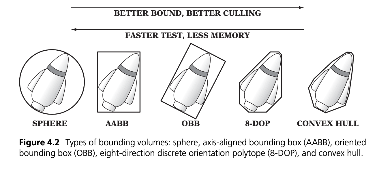
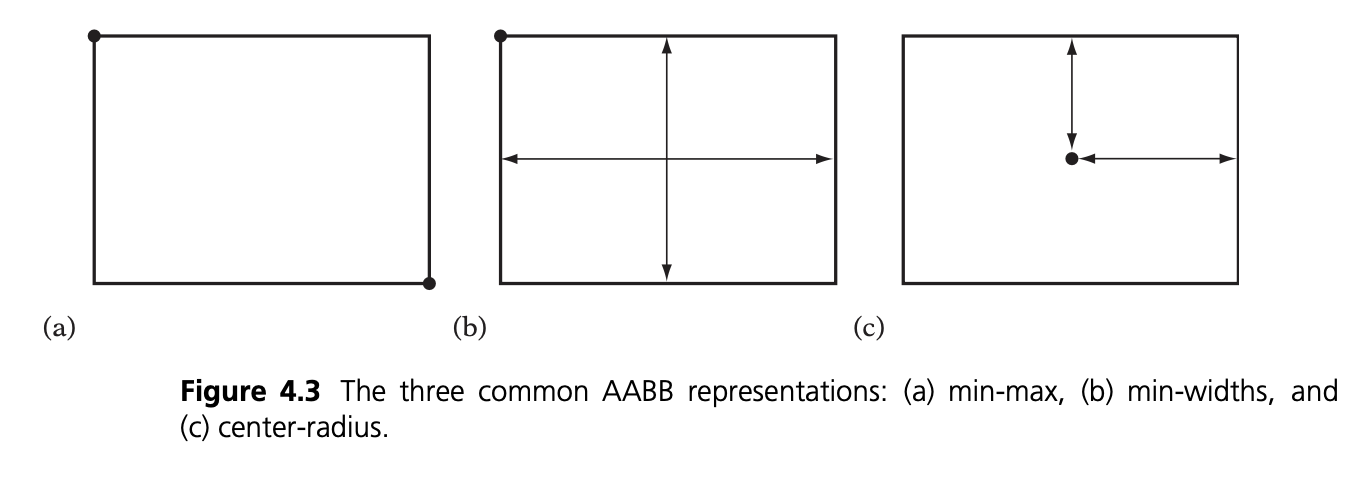
1.1.1. Axis-Aligned Bounding Boxes (AABBs)
There are 3 main manners of defining such boxes. The overlap tests are straightforward: 2 AABBs only overlap if they overlap on all 3 (or 2 in 2D) axes.
But these can very rapidly lead to false results when dealing with more complex shapes, specially when they are close or not aligned with the AABB’s axes, since the overlapp test on the bounding box of one object can be a false-True, meaning it’s possible for the second object to never be tested against rays incomming from the first object’s bounding box.
Such overlapping tests can be done using simple comparisons, as shown in the following code snippet for a min-max 3D representation:
int TestAABBAABB(AABB a, AABB b)
{
    // Exit with no intersection if separated along an axis
	if (a.max[0] < b.min[0] || a.min[0] > b.max[0]) return 0;
	if (a.max[1] < b.min[1] || a.min[1] > b.max[1]) return 0;
	if (a.max[2] < b.min[2] || a.min[2] > b.max[2]) return 0;
	// Overlapping on all axes means AABBs are intersecting
	return 1;
}
Code snippet and previous image from [real-time-collision-detection] by Christer Ericson
1.1.2. Oriented Bounding Boxes (OBBs)
On the other hand, one can use OBBs in order to represent complex or overlapping shapes. Thos are of rectangular shape but try to minimize the volume of the box by aligning it with the object’s orientation. This can be done by using the object’s center point plus an orientation matrix and three halfedge lengths. This way, the box will be as tight as possible around the object, and the overlap tests will be as effective as possible. But this comes at a cost as the overlap tests are more expensive, since many different separating axes must be tested (15 in 3D), and their instanciation is more complex.
But since our discretization is composed of simple shapes, triangles, we used AABBs to optimize the traversal time, since no overlappings are allowed in our meshes.
1.2. Bounding Volume Hierarchy
The construction of an effective and well-optimized Bounding Volume Hierarchy (BVH) plays a pivotal role in determining the efficiency of these calculations. Choosing the right BVH construction algorithm can greatly impact the speed and accuracy of solar shading mask calculations.
Numerous techniques have been developed to construct BVHs efficiently, and the choice of technique can significantly affect the structure and traversal behavior of the resulting BVH. Techniques vary from classic bottom-up approaches like the Surface Area Heuristic (SAH) to top-down techniques like Binary Space Partitioning (BSP).
Each technique has its strengths and weaknesses, and their impact becomes even more pronounced when applied to solar shading mask calculations. For instance, scenes with highly detailed geometry might benefit from BVHs constructed with the SAH algorithm (Cost Functions), as it efficiently reduces the number of unnecessary ray-object intersection tests. On the other hand, scenes with varying object densities could benefit from median splits and axis-cycling, ensuring that the splitting axes are evenly distributed and can help maintain overall balance during the BVH construction.
Furthermore, the trade-off between construction time and traversal efficiency cannot be overlooked. While some techniques may yield BVHs with faster traversal times, they might require longer construction times, but this would be acceptable for the computation of solar shading masks, since the BVH is constructed only once and then used for many ray-object intersection tests.
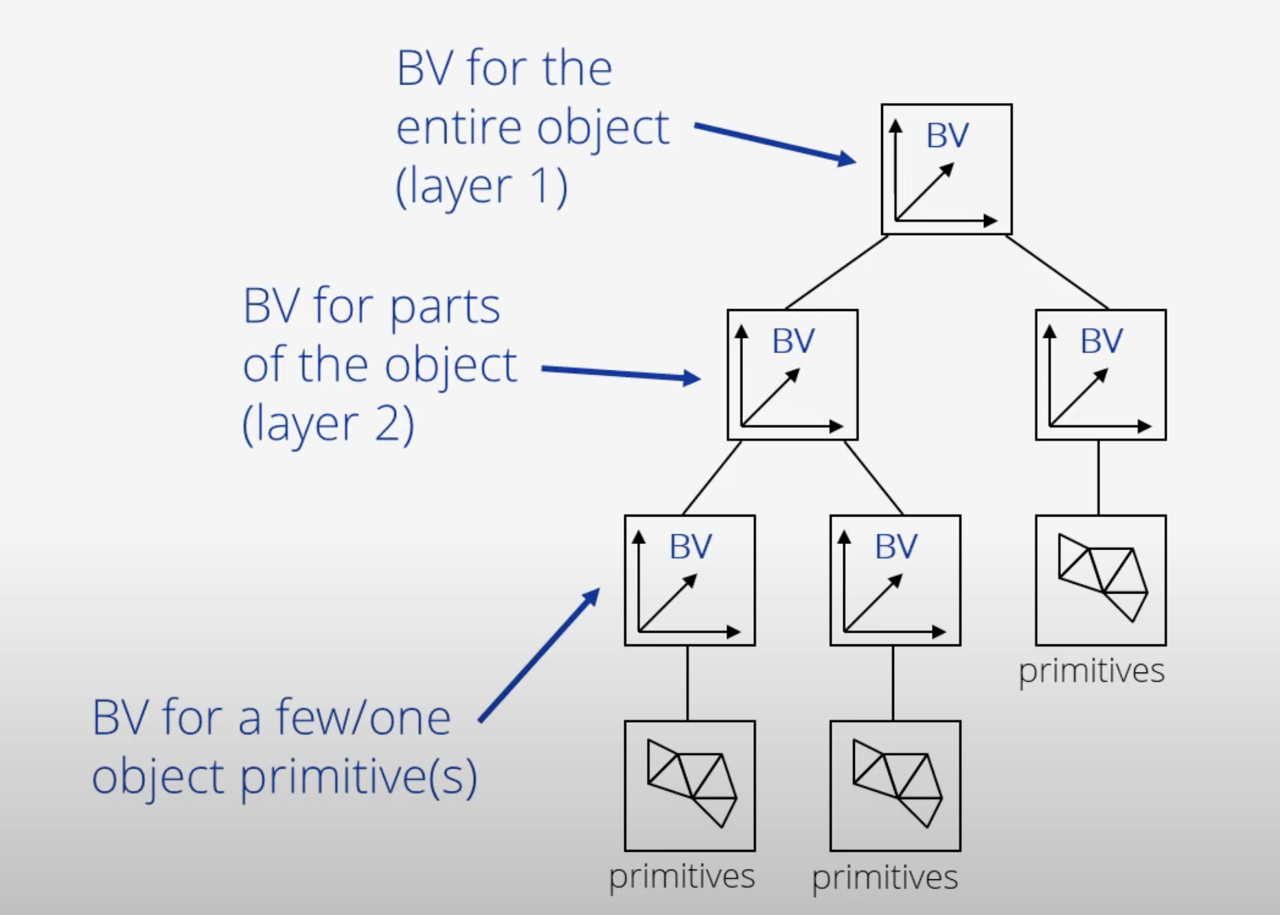
A visual definition of a BVH structure using Axis-Aligned Bounding-Boxes (from here)
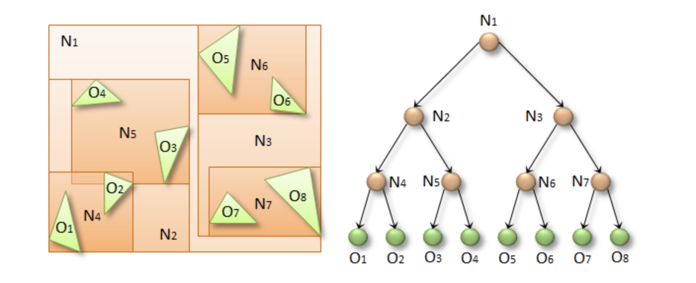
In this context, N1 would be the bounding volume for the entire object or scene, N2 and N3 would be those respectively containing N4 and N5, and so on, until we reach the leaves of the tree, which are directly the bounding boxes of the primitives.
2. Construction
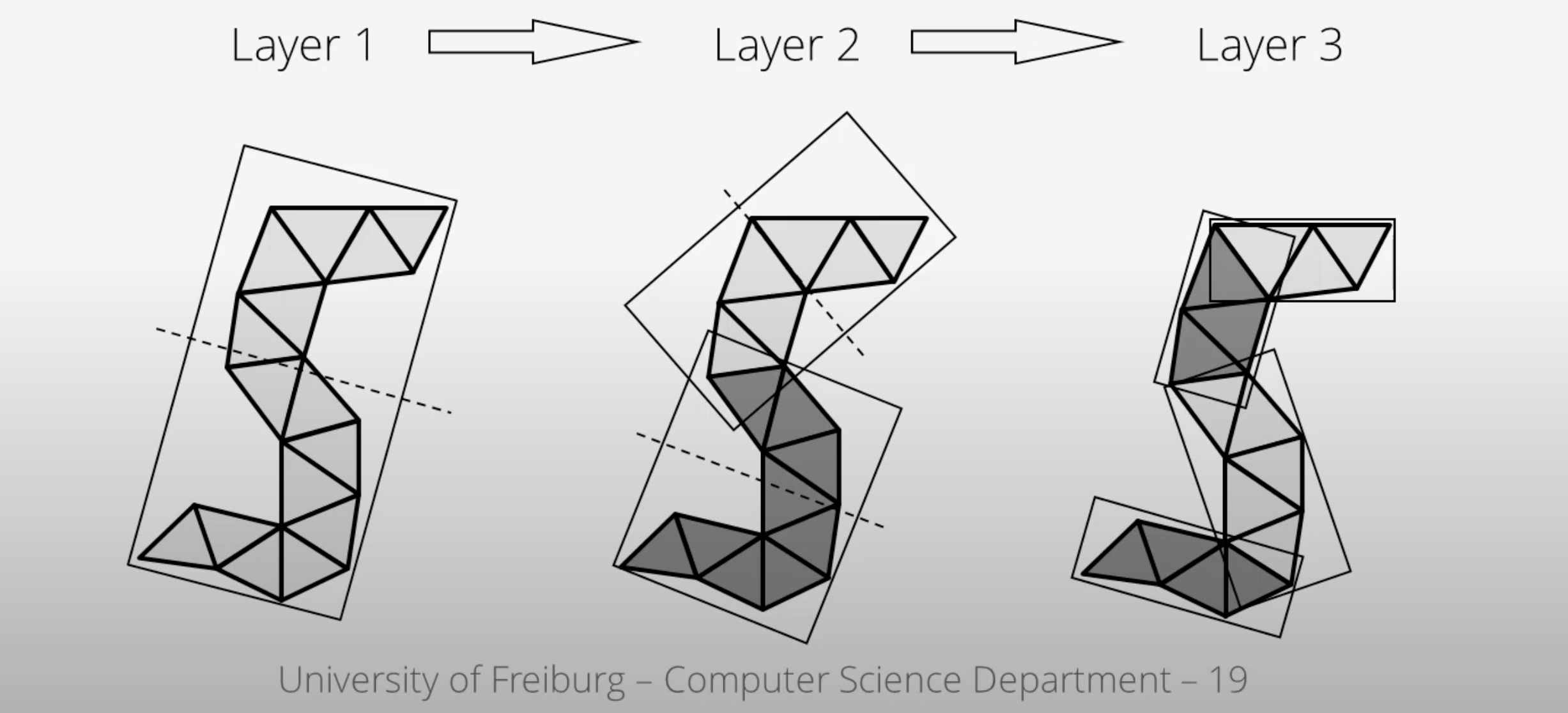
Visual representation of the construction process of a BVH :
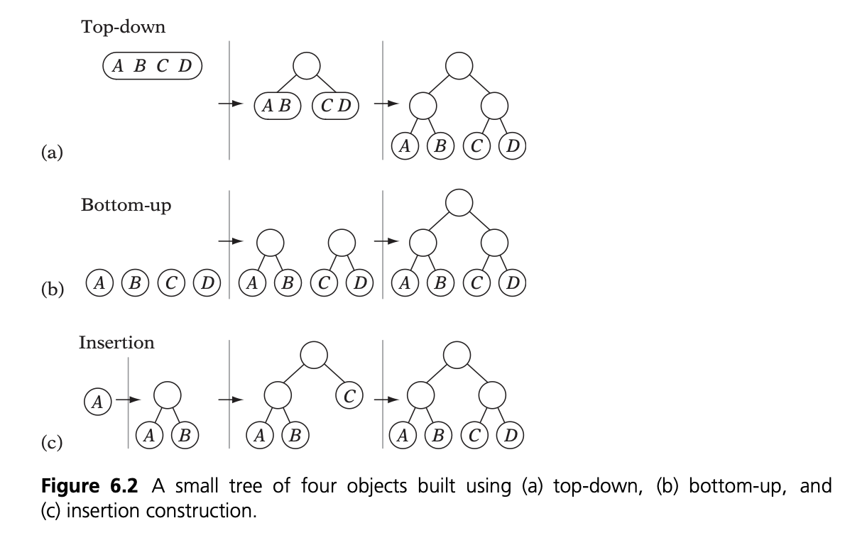
Image coming from [freiburg-lecture-bvh].
2.1. Recursive Top-Down Construction
In the code snippet below, written by Luca Berti, a recursive top-down construction algorithm was proposed for further improvements. We can see that he adopts a recursive build function, which is called to create each node of the tree. Here is the proposed implementation:
    BVHNode * recursiveBuild(BVHNode * current_parent, int cut_dimension, int start_index_primitive, int end_index_primitive, std::vector<int> &orderedPrims)
    {
        LOG(INFO) <<fmt::format("cut dimension {}, start index primitive {}, end index primitive {}",cut_dimension,start_index_primitive,end_index_primitive);
        Eigen::VectorXd M_bound_min_node(nDim),M_bound_max_node(nDim);
        BVHNode * node = new BVHTree::BVHNode();
        M_bound_min_node = M_primitiveInfo[start_index_primitive].M_bound_min;
        M_bound_max_node = M_primitiveInfo[start_index_primitive].M_bound_max;
        for (int i = start_index_primitive+1; i < end_index_primitive; ++i)
		{
            M_bound_min_node = node->newBoundsMin(M_bound_min_node,M_primitiveInfo[i].M_bound_min);
            M_bound_max_node = node->newBoundsMax(M_bound_max_node,M_primitiveInfo[i].M_bound_max);
        }
        auto mid = (start_index_primitive + end_index_primitive) / 2;
        std::nth_element(&M_primitiveInfo[start_index_primitive], &M_primitiveInf[mid], &M_primitiveInfo[end_index_primitive-1]+1,
        [cut_dimension](const BVHPrimitiveInfo &a, const BVHPrimitiveInfo &b)
		{
            return a.M_centroid[cut_dimension] < b.M_centroid[cut_dimension];
        });
        int nPrimitives = end_index_primitive - start_index_primitive;
        if (nPrimitives == 1)
        {
            // Create a leaf, since there is only one primitive in the list
            int firstPrimOffset = orderedPrims.size();
            for (int i = start_index_primitive; i < end_index_primitive; ++i)
            {
            int primNum = M_primitiveInfo[i].M_primitiveNumber;
            orderedPrims.push_back(primNum);
            }
            node->buildLeaf(current_parent,firstPrimOffset, nPrimitives, M_bound_min_node,M_bound_max_node);
            return node;
        }
        else{
            // Create a node, since there are at least two primitives in the list
            node->buildInternalNode(current_parent,(cut_dimension+1)%nDim,
                                    recursiveBuild( node, (cut_dimension+1)%nDim, start_index_primitive, mid, orderedPrims),
                                    recursiveBuild( node, (cut_dimension+1)%nDim, mid, end_index_primitive, orderedPrims));
        }
        return node;
    }
This function is responsible for constructing the BVH tree from the primitives. It’s called recursively and each time it either creates a leaf node if there’s only one primitive left, or an internal node with two child nodes. The primitives are split by choosing a cutting dimension and sorting them by their centroids along this dimension, and then the data is divided into two equally sized parts, for each of which a new node is created.
The cutting dimension is cycled between 0, 1, 2 (representing the x, y, and z axes in a 3D space) by using (cut_dimension+1)%nDim in the recursive calls (Axis Cycling). This is the main "Divide and Conquer" idea behind this top-down construction algorithm.
It then sorts the primitives by their centroids along the cutting dimension, using the std::nth_element function, which partially sorts the primitives so that the element at the mid index will be in the place it would be in a fully sorted array, and all elements before it are less than or equal to the elements after it. The comparison function :
[cut_dimension](const BVHPrimitiveInfo &a, const BVHPrimitiveInfo &b) { return a.M_centroid[cut_dimension] < b.M_centroid[cut_dimension]; }is used to sort the elements based on their centroids along the cutting dimension (Median Cut).
Finally, the data is divided into two equally sized parts when calculating the midpoint of the primitives' indexes.
Other splitting algorithms can be used, such as the Surface Area Heuristic (SAH) or the Middle Split Heuristic (MSH), which are listed and explained in the Spatial Splits and Clustering section.
2.2. Bottom-Up Construction
Instead of starting with all scene primitives in one cluster and recursively splitting them, bottom-up construction algorithms start with each primitive in its own cluster and recursively merge the closest pairs. This is done either until the desired number of clusters is reached, or each cluster contains a maximum number of primitives. The clusters are then used as the primitives for the next level of the tree. This process is repeated until the root node is reached.
But such a method wouldn’t be the best for our purpose, first of all, looking at its inefficiency in finding pairs, we observe that every time we need to merge two clusters, we have to determine which two are the closest. This operation can be computationally expensive and can result in O(n^2) time complexity if not optimized. For a large number of primitives, this can slow down the construction process considerably. Most important, such techniques suffer from a strong lack in flexibility: the algorithm involves the creation and deletion of nodes dynamically, and the management of an array of active nodes. This can lead to fragmentation and additional memory overhead, which is unacceptable due to the need of scaling up the algorithm to be performed on GPUs, where memory is very limited. The bottom-up approach generally lacks the flexibility to adapt the BVH structure based on specific traversal use-cases. For instance, in solar shading masks computations, certain areas might need more detailed BVH structures (higher resolution) than others. Bottom-up methods don’t inherently allow for this granularity during construction, as opposed to the top-down approach, where the BVH structure can be adapted to our needs at each step of the construction process.
Below is an example of a bottom-up construction algorithm, found in [real-time-collision-detection] by Christer Ericson:
Node *BottomUpBVTree(Object object[], int numObjects)
{
    assert(numObjects != 0);
	int i, j;
	// Allocate temporary memory for holding node pointers to // the current set of active nodes (initially the leaves) NodePtr *pNodes = new NodePtr[numObjects];
    // Form the leaf nodes for the given input objects
    for (i = 0; i < numObjects; i++) {
        pNodes[i] = new Node;
        pNodes[i]->type = LEAF;
        pNodes[i]->object = &object[i];
	}
    // Merge pairs together until just the root object left
    while (numObjects > 1) {
        // Find indices of the two "nearest" nodes, based on some criterion
        FindNodesToMerge(&pNodes[0], numObjects, &i, &j);
        // Group nodes i and j together under a new internal node
		Node *pPair = new Node;
		pPair->type = NODE;
		pPair->left = pNodes[i];
		pPair->right = pNodes[j];
		// Compute a bounding volume for the two nodes
		pPair->BV = ComputeBoundingVolume(pNodes[i]->object, pNodes[j]->object);
		// Remove the two nodes from the active set and add in the new node.
		// Done by putting new node at index ’min’ and copying last entry to ’max’ int min = i, max = j;
		if (i > j) min = j, max = i;
		pNodes[min] = pPair;
		pNodes[max] = pNodes[numObjects - 1];
		numObjects--;
	}
    // Free temporary storage and return root of tree
    Node *pRoot = pNodes[0];
    delete pNodes;
    return pRoot;
}
Introduced by Walter et al., bottom-up construction by agglomerative clustering proposes to start with all scene primitives considered as individual clusters and recursively merges the closest pairs (the distance function being for example the surface area of a bounding box enclosing both clusters). In general, these trees tend to have lower global costs, but the construction is more time-consuming.
3. Spatial Splits and Clustering
Performing the spatial splits in an optimized way is crucial to the performance of the BVH. In fact, this is deeply related to the BVH’s layout, which is the way the BVH is stored in memory, hence having a strong impact on it’s construction time, the resulting quality of the BVH, and the traversal performance. The first step is to choose the splitting algorithm, and more importantly the separating axes.
3.1. Morton Curves
-
Morton Curves
These can be defined thanks to various algorithms presented on NVIDIA’s website.
3.2. Agglomerative Clustering
The major inconvenience when using bottom-up algorithms is that the upper nodes are poorly locally optimized and thus the research for the closest neighbor can be very costly. To prevent this, Gu et al proposed to recursively perform spatial median splits based on Morton codes until each subtree contains less than a chosen number of clusters. The clusters are merged using agglomerative clustering. Using this at all levels in the BVH, even the top level nodes' split will be locally optimized.
Meister and Bittner proposed a GPU-based algorithm using k-means clustering (found in [real-time-collision-detection]): scene primitives are subdivided into k clusters using k-means clustering. When done recursively, a k-ary BVH is built, which can also be converted to a binary tree by constructing intermediate levels using agglomerative clustering.
3.3. Parallel locally-ordered clustering on GPU
Introduced by Meister and Bittner, the key observation is that the distance functions have a non-decreasing property, meaning that once we found two mutually corresponding nearest neighbors, we can immediately merge their clusters since no other closer one will be found. The clusters are kept sorted along the Morton Curve, finding the nearest cluster by searching both sides of the sorted cluster array, testing a predefined number of clusters. Since it does not rely on distance matrices, it is GPU-friendly, and only a small number of iterations are needed to build the whole tree.
3.4. Linear BVH (LBVH)
The hierarchical nature of the BVH prevents a straightforward parallelization of the construction algorithm. But now, the BVH construction can be reduced to sorting scene primitives along the Morton curve (the order is given by Morton codes of fixed length, 32 or 64 bits), and using optimized sorting algorithms such as the radix sort, it can be done in 2n-1 time. The Morton code implicitly encodes a BVH constructor by spatial median splits.
3.5. Longest Axis
One straightforward approach is to choose the axis with the longest extent of the bounding volume as the separating axis. This can help effectively divide the scene along its largest dimension, potentially leading to more balanced partitions.
3.6. Axis Cycling
Another method involves cycling through the three axes (X, Y, Z) and selecting the next axis in a cyclic manner for each spatial split. This approach ensures that the splitting axes are evenly distributed and can help maintain overall balance in the BVH construction. This is the approach proposed by Luca Berti, presented in the original code of this project, like seen during the call to the recursive build function:
node->buildInternalNode(current_parent,(cut_dimension+1)%nDim,
                                        recursiveBuild( node, (cut_dimension+1)%nDim, start_index_primitive, mid, orderedPrims),
                                        recursiveBuild( node, (cut_dimension+1)%nDim, mid, end_index_primitive, orderedPrims));
The 2nd value representing the cutting dimension is cycled between 0, 1 and 2, representing the x, y and z axes of our 3 dimensional euclidean space, by using (cut_dimension+1)%nDim in the recursive calls. At each call, it is incremented by 1, enabling a different splitting axis to be used at each level of the tree. After choosing the splitting axis, the median value along that axis is computed and used as the splitting position, also know as a median cut, discussed right below.
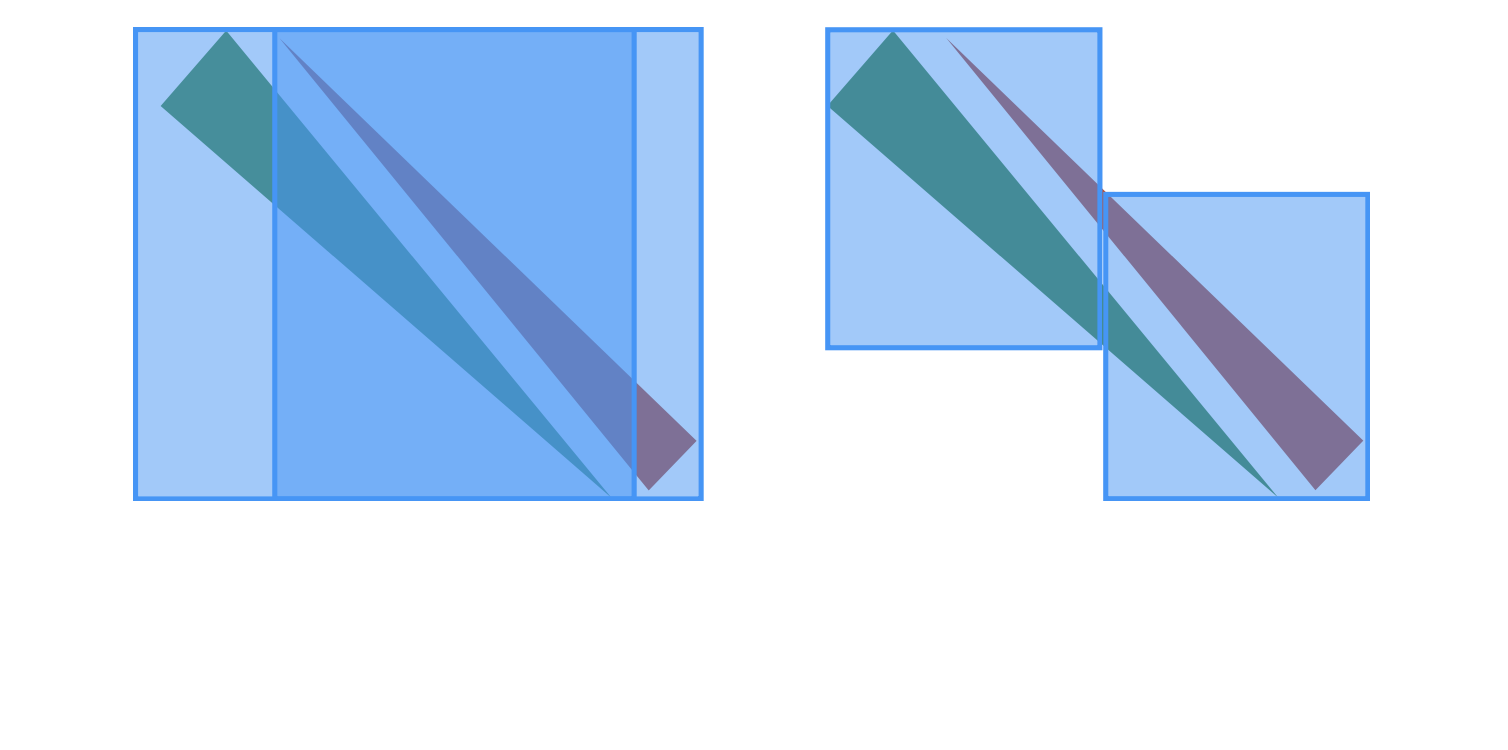
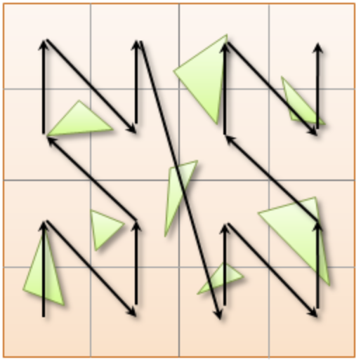
3.7. Median Cut
The median cut strategy involves computing the median value along a specific axis and using it as the splitting position. This method aims to divide the scene into two halves containing an equal number of objects, which can help achieve good load balancing. This is implemented in the following line of the recursive build method, when calling the std::nth_element function:
auto mid = (start_index_primitive + end_index_primitive) / 2;
std::nth_element(&M_primitiveInfo[start_index_primitive], &M_primitiveInfo[mid],
        &M_primitiveInfo[end_index_primitive-1]+1,
            [cut_dimension](const BVHPrimitiveInfo &a, const BVHPrimitiveInfo &b) {
                return a.M_centroid[cut_dimension] < b.M_centroid[cut_dimension];
            });
Here is an example of a construction using the median cut strategy, but on a single splitting axis:
And such spacial divisions can lead to a similar tree as the following:
We will combine this method with the Axis Cycling one, to ensure that the splitting axes are evenly distributed and can help maintain overall balance during the BVH construction.
3.8. Cost Functions
The quality of a particular BVH can be estimated in terms of the expected number of operations needed for finding the nearest intersection with a given ray. It can be estimated thanks to the recurrence equation according to Daniel Meister et al. [survey-BVHs-for-ray-tracing]:
3.8.1. Surface Area Heuristic (SAH)
As mentioned earlier, the SAH criterion can also be used to determine the separating axis. It evaluates the cost of each axis based on the surface area of the resulting bounding volumes and chooses the axis with the lowest cost.
Using the surface area heuristic (SAH), we can express the conditional probabilities as geometric ones, using their respective surface area to compute the ratio of the surface areas of a child node and the parent’s one:
And finally, assuming that the ray origins and directions are uniformly distributed, after unrolling we get:
Where \(N_i\) and \(N_l\) respectively denote interior and leaf nodes of a subtree with root \(N\). The problem of finding an optimal BVH is believed to be NP-hard. But these assumptions are unrealistic and thus several corrections have been proposed.
4. Layout
After successfully constructing the tree in an optimized way, it is important to note that both optimizing the traversal code and the tree’s representation itself are very important to see an increase in performance. Two obvious ways of dealing with that are to minimize the size of the data structures involved and to rearrange the data in a more cache-friendly way to reduce time for the search of relevant information (for example, it would be better to structure the array holding the pointers in such a way to minimize the time spent during traversal). Most of the information in this part comes from the book [real-time-collision-detection] by Christer Ericson (namely all images used in this section).
4.1. Array Representation
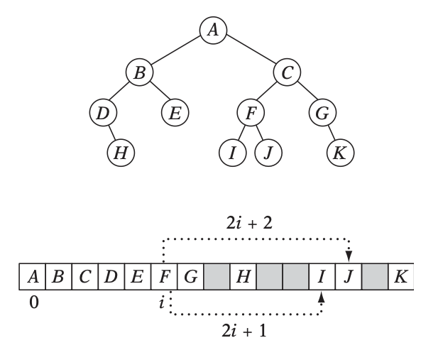
Let’s look at a natural way of structuring the tree by mapping its nodes in a breadth-first level-by-level manner:
// First Level
array[0] = *(root);
// Second level
array[1] = *(root->left);
array[2] = *(root->right);
// Third level
array[3] = *(root->left->left);
This way, we always know that a parent’s children can be found at positions \(2i+1\) and \(2i+2\) in the array, usually inducing wasted memory unless dealing with a complete tree.
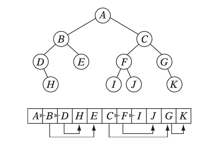
4.2. Preorder Traversal Order
When preordering them in traversal order, the left child will always follow its parent, and only one link is needed to point to the right child.
// Given a tree t, outputs its nodes in preorder traversal order
// into the node array n. Call with i = 0.
int PreorderOutput(Tree *t, Tree n[], int i)
	{
	// Implement a simple stack of parent nodes.
	// Note that the stack pointer ‘sp’ is automatically reset between calls
	const int STACK_SIZE = 100;
	static int parentStack[STACK_SIZE];
	static int sp = 0;
	// Copy over contents from tree node to PTO tree
	n[i].nodeData = t->nodeData;
	// Set the flag indicating whether there is a left child
	n[i].hasLeft = t->left != NULL;
	// If node has a right child, push its index for backpatching
	if (t->right) {
		assert(sp < STACK_SIZE);
		parentStack[sp++] = i;
	}
	// Now recurse over the left part of the tree
	if (t->left)
		i = PreorderOutput(t->left, n, i + 1);
	if (t->right) {
		// Backpatch the right-link of the parent to point to this node
		int p = parentStack[--sp];
		n[p].rightPtr = &n[i + 1];
		// Recurse over the right part of the tree
		i = PreorderOutput(t->right, n, i + 1);
	}
	// Return the updated array index on exit
	return i;
}
Flattening the tree in this way allows us to store the tree in a single array, with each node containing a pointer to its right child and a flag indicating whether it has a left child or not. This way, we can easily traverse the tree by following the right child pointers and using the left child flags to determine whether we should follow the left child or not and avoid the need for a stack and storage of 2 pointers per node (only one is necessary). This method is also cache-friendly since the nodes are stored in a linear array.
4.3. Cache-friendly Structures
When using modern architecture, execution time is mostly limited by cache issues when fetching data from memory. One possible way of adopting a cache-friendlier solution would be by merging the sets of binary tree nodes into a 'tri-node' containing the parent and its children, preventing it from needing internal links. Below we can see an example representing a complete 4-level binary tree with 14 internal links with a 2-level tri-node tree storing only 4 internal links. Even better, this representation can also be combined with other optimizing structures seen before.
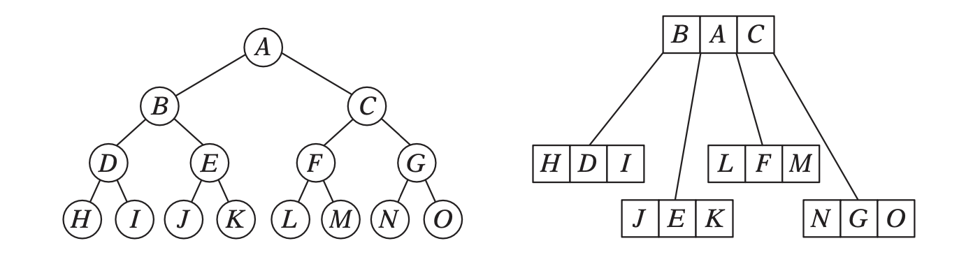
Flattening a tri-node tree is similar to flattening a binary tree, except that we need to store the parent’s index in the array as well as the left and right child flags. The right child pointer is replaced by a flag indicating whether the parent has a right child or not, the left and parent’s one are replaced in the same manner. The root node is a special case, since it has no parent, signified by a special flag. Three new structures (GPUNode, GPURay and GPUTree) were introduced, storing only critical information for it to be of small enough size to be copied-by-value to the GPU.
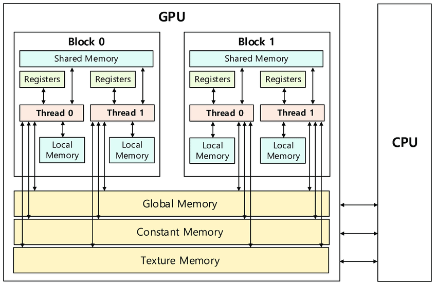
4.4. GPU Implementation
In our own GPU implementation, which had to be able to reproduce exactly the same BVHs as the original one presented by Luca Berti, we had no other choice than copying the informations containend in each BVH node to the GPU, and force it to retain the exact same structure. In order to do so, a suitable structure for the rays, the nodes and the global BVH had to be found, meaning excluding every unsupported data structure, such as std::vector or Eigen::MatrixXd. The whole BVH had to be flattened into a single static array, preventing different threads to have to access shared memory, which would have been very costly. In order to do so, the following structures where chosen (available in the Bvh_GPU.cuh file):
struct GPURay
{
    float origin[3];
    float dir[3];
};

struct GPUNode
{
    GPUNode* parent;
    GPUNode* leftchild;
    GPUNode* rightchild;
    int nPrimitives;
    int firstPrimOffset;
    int splitAxis;
    float bounds_min[3];
    float bounds_max[3];
    float centroid[3];
};

struct GPUBVH
{
    GPUNode* M_root_gpu_tree;
};
And implementing only the methods necessary to perform the basic traversal on the axis-aligned bounding boxes, and not directly on the primitives, which could cause memory overhead.
Looking at the sizes of the differents structures and classes, we can compute the average size of a BVH node (supposing a 64 bits architecture):
-
parent: 8 bytes (double)
-
leftchild: 8 bytes (double)
-
rightchild: 8 bytes (double)
-
nPrimitives: 4 bytes (int)
-
firstPrimOffset: 4 bytes (int)
-
splitAxis: 4 bytes (int)
-
All
Eigen::VectorXdare dynamic-sized vectors, meaning the three M_bound_min, M_bound_max and M_centroid contain the following data: -
size: 4 bytes (int)
-
pointer to data: 8 bytes (double on a 64 bits architecture)
-
the data itself: 3 x 8 bytes (since we are computing the shading mask in 3D)
Total size for BVH Node: 8 + 8 + 8 + 4 + 4 + 4 + 3 x (4 + 8 + 3 x 8) = 144 bytes
Having to transfer \(144 \times N_{nodes}\) could cause memory overhead, contrary to the structure implemented for the GPU:
-
parent: 8 bytes
-
leftchild: 8 bytes
-
rightchild: 8 bytes
-
nPrimitives: 4 bytes
-
firstPrimOffset: 4 bytes
-
splitAxis: 4 bytes
-
bounds_min: 3 x 4 = 12 bytes
-
bounds_max: 3 x 4 = 12 bytes
-
centroid: 3 x 4 = 12 bytes
Which totals out at 72 bytes per node, which is half the size of the original structure, and thus much more efficient in terms of memory usage. This enables us also to be able to create pointers on the GPU to perform the stack-less traversal without the need of preordering the nodes in a specific order such as described in the Preordering Algorithm section.
5. Traversal
5.1. Stack-Based Algorithms
5.1.1. Definition
Stack-based algorithms for ray traversal through a bounding volume hierarchy (BVH) conventionally employ a stack to maintain the traversal state of the ray through the hierarchy. Unlike their stack-less counterparts, these algorithms do not require frequent restarts of the traversal from the root nor traverse more nodes. The use of a stack to save traversal states aids in efficiently determining the next node to be visited, enabling a more straightforward path through the hierarchy. Although stack operations (push and pop) might sound costly, their implementation on modern architectures, even GPUs, is quite efficient, especially when balanced against the potential overhead of other traversal techniques. The primary benefits of a stack-based algorithm include: - Speed: Generally faster than their stack-less counterparts, especially for balanced BVHs, as there are fewer extraneous operations and more direct traversal paths. - Simplicity: The algorithm’s structure is more intuitive, which often leads to simpler code and fewer bugs. - Flexibility: Easy adjustments can be made for different traversal strategies or optimizations.
However, stack-based methods might suffer from memory overhead due to the need of a stack to store traversal states, which could be prohibitive in highly parallel environments, like GPUs, with limited shared memory. Additionally, when working with such algorithm, one can encounter parallelisation limitations, in fact, the push and pop operations on a shared stack can become bottlenecks in highly parallel systems (can be overcome by using atomic counters, available when working with CUDA).
5.1.2. Algorithm
For a clear understanding of the stack-based approach, we can draw an analogy with a depth-first search (DFS) in graph theory, where a stack keeps track of nodes yet to be explored. Here’s a basic pseudocode for the stack-based traversal (found in [real-time-collision-detection]):
struct StackItem {
	Node* node;
	float tmin, tmax; // ray's parametric range for this node
};

void traverseStackBased(ray) {
	StackItem stack[MAX_DEPTH];
	int stackPointer = -1;

	stack[++stackPointer] = {root, 0, INFINITY}; // Push root to the stack

	while (stackPointer >= 0) {
		StackItem current = stack[stackPointer--]; // Pop the top item

		if (boxtest(ray, current.node, current.tmin, current.tmax) != MISSED) {
			if (isLeaf(current.node)) {
				// ray-primitive intersection tests
				processLeaf(ray, current.node);
			} else {
				// Determine near and far child based on ray direction or other criteria
				Node* nearChild = getNearChild(current.node, ray);
				Node* farChild = getFarChild(current.node, ray);

				// Push children onto the stack
				stack[++stackPointer] = {farChild, current.tmin, current.tmax};
				stack[++stackPointer] = {nearChild, current.tmin, current.tmax};
			}
		}
	}
}
This approach showcases the power of the stack in maintaining traversal state, providing a more direct and efficient path through the BVH.
5.2. Stack-Less Algorithms
5.2.1. Definition
Traversing a ray through a bounding volume hierarchy is usually carried out in a recursive manner, therefore making it maintain a full stack per ray, which rapidly becomes very costly. Several stack-less algorithms exist, however they have to perform frequent restarts of the traversal from the root or traverse more nodes than their stack-based counterparts.
Many reasons have pushed researches in this field, such as:
-
efficient memory usage: since stack-less algorithms don’t require keeping track of the traversal state. This is critical when implementing it on GPUs, where memory is very limited
-
parallelism: since they do not require to push and pop from a stack, these methods offer rich parallelization capabilities
The presented algorithm presents a stack-less iterative method traversing the BVH structure in the exact same order as stack-based ones, mainly thanks to added parent-pointers stored within each node and thus performing only one ray-box intersection test per internal node.
5.2.2. Assumptions to be made
-
use of a binary BVH, in which all primitives are stored in leaf nodes, and in which each inner node has exactly two children (so-called siblings)
-
there is an efficient way of determining each node’s parent and sibling
-
for each inner node there is a unique traversal order in which it’s children are traversed, possibly varying from ray to ray.
5.2.3. Algorithm
A commonly-used way of storing the parent’s information is to store an explicit parent pointer for each node, done either by squeezing the parent pointer into unused parts of the node or by storing them directly in a separate array of parent pointers.
For traversal order, a first method would be to store for each node the coordinate axis along which the builder split the parent node and use the ray’s direction sign in this dimension to determine the traversal order. On the other hand, we can directly use the dimension in which the nodes' centroids are widest apart. Finally, we could also directly compute the distance to the sibling’s bounding boxes, inferring many computations.
First, in order to fully understand the methods benefits, let us understand all the underlyings of recursive algorithms.After having successfully intersected the parent, the traversal goes to the nearChild (found with any type of method), and does a ray-box test for this node. If the node is missed, farChild is processed, But if the test was successful, it continues by intersecting its primitives (if the node is a leaf), or by recursively entering the node’s subtree (in case it’s an inner node). Once nearChild is fully processed, traversal resumes with farChild exactly and the same sequence of events takes place.
This already gives us an overlook of the deterministic automaton algorithm (pseudo-code available in "Efficient Stack-less BVH Traversal for Ray Tracing"). In fact, we can start and make a parallel between the three ways of how any given node can be traversed and the tree states of the algorithm. During recursive traversal, a node can either be traversed:
- from its parents (case fromParent): we know that we are entering nearChild. We traverse the current node: if it’s missed, we proceed with a fromSibling case and if not, either it’s a leaf node and we intersect its primitives, or it’s an inner node and we continue with its subtree.
- from its siblings (case fromSibling): we are entering farChild and we are traversing this node for the first time. If it’s missed, we back-track to its parent. Otherwise we intersect it’s primitives against the ray if it’s a leaf node and proceed to parent, and if not we enter the current node’s subtree performing a fromParent step.
- from one of its children (case fromChild): the current node was already tested during the top to bottom phase, it should not be re-tested. The next on the list is either the current node’s farChild or its parent
Algorithm Developed by the Authors (Michal Hapala, Tomas Davidovic, Ingo Wald, Vlastimil Havran and Philipp Slusallek) of the article Efficient Stack-less BVH Traversal for Ray Tracing [efficient-stackless-bvh-traversal] further implemented by Luca Berti in the original code of this project:
void traverse(ray, node) {
	char state = fromParent;
	while (true) {
		switch (state) {
			case fromChild:
				if (current == root) return; // finished
				if (current == nearChild(parent(current))){
					current = sibling(current);
					state = fromSibling; // (1a)
				}
				else {
					current = parent(current);
					state = fromChild; // (1b)
				}
				break;
			case fromSibling:
				if (boxtest(ray, current) == MISSED) {
					current = parent(current);
					state = fromChild; // (2a)
					}
				else if (isLeaf(current)) {
					// ray-primite intersection tests
					processLeaf(ray, current);
					current = parent(current);
					state = fromChild; // (2b)
				}
				else {
					current = nearChild(current);
					state = fromParent; //2a
				}
				break;
			case fromParent:
				if (boxtest(ray, current) == MISSED) {
					current = sibling(current);
					state. = fromSibling; // (3a)
				}
				else if (isLeaf(current)) {
					// ray-primitive intersection tests
					processLeaf(current);
					current = sibling(current);
					state = fromSibling; // (3b)
				}
				else {
					current = nearChild(current);
					state = fromParent; // (3a)
				}
				break;
		}
	}
}
This algorithm was also implemented on GPU using CUDA, only performing basic intersection tests on the axis-aligned bounding boxes, and is discussed in the section State-Based GPU Algorithm.
5.3. State-Based GPU Algorithm
When looking at the storage needed for the computation of ShadingMasks, we can pass the whole BVH structure and make a copy of it directly on the GPU’s shared memory. This way, we can avoid the need to transfer the BVH structure from the CPU to the GPU constantly, which can be a very expensive operation. Using such a method may cause problems depending on the size of the BVH structure, since the GPU’s shared memory is limited. However, we can use the its structure’s size as a parameter to determine whether or not we should use this method. If the BVH structure is too big, we can implement smaller structures to hold the BVH, preordering the nodes in flattened 1D array’s only containing useful information (and not all methods and attributes of the BVH structure). This way, we can reduce the size of the BVH structure and make it fit in the GPU’s shared memory. And since the traversal is performed nRays * nElements times (more than 5000 rays per element), we can compute the array’s once by indexing the nodes, its children and its parent.
Depending on the number of bounding boxes representing the acceleration structure, we can use the same stack-less algorithm as used on the CPU before, only adding atomic operations to count the number of intersections between a certain ray and leaf nodes. If a leaf is intersection, we append the firstPrimOffset to the results list, enabling the CPU to access the primitives and perform the intersection tests. This way, we avoid the need to transfer twice the amount of data.
__device__ void GPU_traverse_stackless(GPUNode * tree, GPURay const& ray, int * results, int & result_count)
{
	auto current_node = tree -> nearChild(ray);
	char state = 'P';

	result_count = 0;

	while (true)
	{
		switch (state)
		{
			case 'C':
				if (current_node == M_root_gpu_tree) return;

				if (current_node == current_node->parent->nearChild(ray))
				{
					current_node = current_node->otherChild(current_node->parent);
					state = 'S'; // from Sibling
				}
				else
				{
					current_node = current_node->parent;
					state = 'C'; // the current node has been accessed from its sibling
				}
				break;

			case 'S': // the node is being traversed from its sibling
				if (current_node->checkintersection(ray)==false) // go back to parent
				{
						current_node = current_node->parent;
					state = 'C';
				}
				else if (current_node->isLeaf())
				{
					int index = atomicAdd(&result_count, 1);
					results[index] = current_node->getfirstPrimOffset();// multiple threads try to write to the same index, we will not lose any results since they'll be queued
					current_node = current_node->parent;
					state = 'C';
				}
				else
				{
					current_node = current_node->parent;
					state = 'P';
				}
				break;

			case 'P':
				if (current_node->checkIntersection(ray)==false)
				{
					current_node = current_node->otherChild(current_node->parent);
					state = 'S';
				}
				else if (current_node->isLeaf())
				{
					int index = atomicAdd(&result_count, 1); // Increment the result_count atomically and get the previous value as the index
					results[index] = current_node->getfirstPrimOffset();
					current_node = current_node->otherChild(current_node->parent);
					state = 'S';
				}
				else
				{
					current_node = current_node->nearChild(ray);
					state = 'P';
				}
				break;

			default:

				break;
		}
	}
}
This method can be coupled with different parallelization methods, since it serves a more generall purpose, namely the traversal of the BVH structure by a single ray. Leveraging the GPU’s parallelization capabilities, we can write a kernel that will be executed by all the available threads, each one performing the traversal of a single ray.
|
The number of intersections we can have per ray had to be limited (here 10) because of the limited size of the shared memory. Using dynamic memory allocation is infeasible due to significant runtime delays. |
__global__ void GPU_traverse_kernel(GPUNode* tree, GPURay const* rays, int* results, int numRays)
{
	int index = threadIdx.x + blockIdx.x * blockDim.x;
	int N = 10 ; // this is the max number of intersections we can have per ray
	if (index < numRays)
	{
		int thread_results[N]; // Local array specific to each thread
		int result_count = 0; // Local variable specific to each thread
		GPU_traverse_stackless(tree, rays[index], thread_results, result_count);

		for (int i = 0; i < result_count; i++)
		{
			results[index * 10 + i] = thread_results[i]; // Store results in the global results array
		}
	}
}
In this implementation, each thread is assigned a single ray and will perform the traversal of the BVH structure, storing the results in a local array. Once the traversal is done, the results are stored in the global results array, which will be accessed by the CPU to perform the intersection tests on the primitives.
Finally, the last parallelization occurs when the wrapper method calls the GPUraySearch method, which will be executed on all available GPUs in the cluster, each one maxing out their number of threads.
__host__ std::vector<int> GPUraySearch(std::vector<Feel::BVHRay> const& rays, const Feel::BVHTree<3> * tree)
{
	int totalRays = rays.size();
	int numDevices;
	CHECK_CUDA_ERRORS(cudaGetDeviceCount(&numDevices));
	int raysPerDevice = totalRays / numDevices; // Assuming totalRays is divisible by numDevices here.
	std::vector<double> lengths; // no distances are computed on the GPU
	std::vector<GPURay> rayons;
	std::vector<int> results(totalRays, -2);

	// convert the BVHRays to GPURays here
	for (int i = 0; i < totalRays; i++)
	{
		rayons.push_back(GPURay(rays[i]));
	}

	// Get all informations on the devices needed to perform the ray search
	cudaDeviceProp prop;
	cudaGetDeviceProperties(&prop, 0);// Assumes all devices are identical
	int maxThreadsDim = prop.maxThreadsDim[0];
	int maxGridSize = prop.maxGridSize[0];
	int maxThreadsPerBlock = prop.maxThreadsPerBlock;
	size_t totalGlobalMem = prop.totalGlobalMem;// Total global memory (in bytes) ===> can be used to check whether the tree fits in the GPU memory
	int threadsPerBlock = std::min(totalRays, maxThreadsPerBlock);
	int blocks = (totalRays + threadsPerBlock - 1) / threadsPerBlock;
	int blocksPerGrid = (raysPerDevice + threadsPerBlock - 1) / threadsPerBlock; // Round up division

	M_root_gpu_tree = buildRootTree(tree);


	cudaStream_t stream[numDevices];
	GPUNode *d_tree[numDevices];
	GPURay *d_rays[numDevices];
	int *d_results[numDevices];

	for (int i = 0; i < numDevices; i++) {
		CHECK_CUDA_ERRORS(cudaSetDevice(i));
		CHECK_CUDA_ERRORS(cudaStreamCreate(&stream[i]));

		// Allocate device memory for rays and copy from host to device
		CHECK_CUDA_ERRORS(cudaMalloc(&d_rays[i], sizeof(GPURay) * raysPerDevice));
		CHECK_CUDA_ERRORS(cudaMemcpyAsync(d_rays[i], rayons.data() + i * raysPerDevice, sizeof(GPURay) * raysPerDevice, cudaMemcpyHostToDevice, stream[i]));

		CHECK_CUDA_ERRORS(cudaMalloc(&d_results[i], sizeof(int) * raysPerDevice));

		d_tree[i] = M_root_gpu_tree->DeepCopy(M_root_gpu_tree);

		// Launch the kernel with one block per ray
		GPU_traverse_kernel<<<blocksPerGrid, threadsPerBlock>>>(d_tree[i], d_rays[i], d_results[i], raysPerDevice);

		// Copy back results, the first fustrum wil be place from results[0] to results[raysPerDevice - 1] and so on
		CHECK_CUDA_ERRORS(cudaMemcpyAsync(results.data() + i * raysPerDevice, d_results[i], sizeof(int) * raysPerDevice, cudaMemcpyDeviceToHost, stream[i]));
	}

	for (int i = 0; i < numDevices; i++)
	{
		CHECK_CUDA_ERRORS(cudaSetDevice(i));
		CHECK_CUDA_ERRORS(cudaStreamSynchronize(stream[i]));
		CHECK_CUDA_ERRORS(cudaStreamDestroy(stream[i]));
		CHECK_CUDA_ERRORS(cudaFree(d_tree[i]));
		CHECK_CUDA_ERRORS(cudaFree(d_rays[i]));
		CHECK_CUDA_ERRORS(cudaFree(d_results[i]));
	}

	return results;
}
In order to take further this work, one could enlarge the last method to take into account different GPU models, each one having a specific amount of memory and threads available. This way, we could optimize the number of rays per device, and thus the number of threads per block, to maximize the number of rays processed per second.
Further optimizations can be made by assigning different parts of the shading mask matrix to different GPUs or threads, which would enable the processing of very large meshes, unable to fit into on single GPU’s memory. Problems at the boundaries (buildings from zone A casting shadows on zone B) could be solved by using a buffer zone, which would be computed by the CPU and then sent to the GPU to be processed, or simply by limiting the origin of the rays to the zone’s boundaries but not the rays' directions (which would specifically cause problems in this case).
5.3.1. Copy-by-value
As presented on NVIDIA’s website, we can directly create a copy of the wanted BVH structure, enabling it to be able to access all needed functions preceded with device. If the memory allows it we can use the state-based traversal algorithm presented above, or use NVIDIA’s iterative traversal method:
__device__ void traverseIterative( CollisionList& list,
                                   BVH& bvh,
                                   AABB& queryAABB,
                                   int queryObjectIdx)
{
    // Allocate traversal stack from thread-local memory,
    // and push NULL to indicate that there are no postponed nodes.
    NodePtr stack[64];
    NodePtr* stackPtr = stack;
    *stackPtr++ = NULL; // push

    // Traverse nodes starting from the root.
    NodePtr node = bvh.getRoot();
    do
    {
        // Check each child node for overlap.
        NodePtr childL = bvh.getLeftChild(node);
        NodePtr childR = bvh.getRightChild(node);
        bool overlapL = ( checkOverlap(queryAABB,
                                       bvh.getAABB(childL)) );
        bool overlapR = ( checkOverlap(queryAABB,
                                       bvh.getAABB(childR)) );

        // Query overlaps a leaf node => report collision.
        if (overlapL && bvh.isLeaf(childL))
            list.add(queryObjectIdx, bvh.getObjectIdx(childL));

        if (overlapR && bvh.isLeaf(childR))
            list.add(queryObjectIdx, bvh.getObjectIdx(childR));

        // Query overlaps an internal node => traverse.
        bool traverseL = (overlapL && !bvh.isLeaf(childL));
        bool traverseR = (overlapR && !bvh.isLeaf(childR));

        if (!traverseL && !traverseR)
            node = *--stackPtr; // pop
        else
        {
            node = (traverseL) ? childL : childR;
            if (traverseL && traverseR)
                *stackPtr++ = childR; // push
        }
    }
    while (node != NULL);
}
But we will optimize it by using the state-based traversal algorithm presented above. Implementing it in CUDA will be similar, leveraging the complex BVH structure containing all the needed functions and attributes.
5.3.2. Preordering Algorithm
If the memory is not big enough to store the whole BVH structure, we can use a preordering algorithm to store the BVH structure in a flattened 1D array. This way, we can store only the needed information for the traversal, and not the whole BVH structure. This method is presented in 'Real-Time Collision Detection' by Christer Ericson. The algorithm is as follows:
int PreorderOutput(Tree *t, Tree n[], int i)
{
	// Implement a simple stack of parent nodes.
	// Note that the stack pointer ‘sp’ is automatically reset between calls
	const int STACK_SIZE = 100;
	static int parentStack[STACK_SIZE];
	static int sp = 0;
	// Copy over contents from tree node to PTO tree
	n[i].nodeData = t->nodeData;
	// Set the flag indicating whether there is a left child
	n[i].hasLeft = t->left != NULL;
	// If node has right child, push its index for backpatching
	if (t->right) {
		assert(sp < STACK_SIZE);
		parentStack[sp++] = i;
	}
	// Now recurse over left part of tree
	if (t->left)
		i = PreorderOutput(t->left, n, i + 1);
	if (t->right) {
		// Backpatch right-link of parent to point to this node
		int p = parentStack[--sp];
		n[p].rightPtr = &n[i + 1];
		// Recurse over right part of tree
		i = PreorderOutput(t->right, n, i + 1);
	}
	// Return the updated array index on exit
	return i;
}

struct Tree {
	NodeData nodeData;
	bool hasLeft;
	Tree *rightPtr;
};
A stack is only used once, in order to identify the order of traversal, but will never be used on GPUs.
This representation also leverages the use of pointers, only using one to point to the right child, which would be accessed only later during traversal since we use a depth-first search if the intersection test was successful for a given node.
5.4. Conclusion
When dealing with the computation of shading masks, view factors or radiative transport, we use static geometry to realistically represent the scene. Only few topological changes have to be taken into account, hence the decision of also optimizing the build for the BVH tree’s quality in order to reduce traversal operations. Even if the construction speed is important, we are not developing a real-time application, but rather trying to compute physically realistic results. We can build the BVH once and reuse it for multiple ray tracing operations without the need to update or rebuild the BVH. This approach can significantly improve performance, as constructing the BVH is a computationally expensive operation.
Even when taking into account the changes occurring due to the seasonality of the chosen districts and cities (french cities are subdued to changing weather conditions, leaves are falling and trees do not cast as big of a shadow in winter than in summer).
6. Optimization
6.1. Software
With its sole focus on accelerating ray tracing on GPUs, NVIDIA’s OptiX API offers a suite of capabilities that often outshines traditional hand-crafted traversal algorithms. We will discuss the inner workings of OptiX, its advantages, and how it can be harnessed to achieve better results.
6.1.1. The Speed Factor of OptiX
Its foundation is built purely for ray tracing operations, allowing it to fine-tune both hardware and software optimizations suited for this task. Being a brainchild of NVIDIA means OptiX gets intimate access to all the unique features and capabilities of NVIDIA GPUs.
At its core, OptiX employs advanced tools such as Bounding Volume Hierarchies and various other data structures optimized for ray tracing, actively diminishing the need for excessive ray-primitive tests.
6.1.2. Speculative Traversal
Imagine a scenario where multiple ray paths are processed all at once, even if eventually, some might not be needed. This concept, known as speculative traversal, shines brightly in the SIMT (Single Instruction, Multiple Threads) or SIMD (Single Instruction, Multiple Data) realms. With multiple units working in tandem, all executing the same operation but on varied data: When a ray hits a decision point within an acceleration structure, like a node in the BVH, it doesn’t just pick one way, it speculatively chooses all possible paths. This approach keeps NVIDIA GPUs, which operate on SIMT/SIMD architectures, active at all time. Different threads or lanes work on different paths concurrently, maximizing throughput. As paths are traversed, the unnecessary ones—like those not intersecting with any primitives in a BVH section—get discarded, paving the way for more essential operations (see Stanford’s lecture on optix [stanford-lecture-optix] for more details)
This method is akin to casting a wide net, ensuring that all possible paths are explored, then discarding the unnecessary ones.
OptiX isn’t just about speed, it enhences the results quality too. For those already familiar with CUDA, OptiX seamlessly meshes with it. This synergy allows for the creation of hybrid solutions, capitalizing on OptiX’s performance and Cuda’s flexibility.
6.2. Hardware
Spatial data structures exploit the spatial locality of scene primitives. But this isn’t the only way of leveraging spatial locality. To further accelerate the whole process, we could map rays to interior nodes deeper in the tree during the traversal, skipping top-level nodes. A major caveat of such methods is that there is no guarantee that the found intersection corresponds to the closest one. But when computing shading masks, the lack of distance consideration is not a drawback. Instead, we solely focus on determining whether an object is present along the path of the ray.
Another way to optimize the ray generation would be to exploit the graphics card’s instancing of objects, enabling it to create multiple copies of one object in record time. Benthin and Wald decided that, instead of tracing the rays sequentially, they would generate bounding frusta of coherent rays simultaneously harnessing the potential of a SIMD unit (as many rays in one frustum as the SIMD unit is wide).
This could be taken further, by assigning parts of a matrix to a specific block in the GPU, leveraging the constant memory and launching the frustum of rays in the respective direction defined by the block-assigned resulting matrix. This way, the rays are processed in a more coherent manner, and the GPU’s constant memory is used to its full potential. Moreover, the frustum could be instantiated directly on the GPU, and the identical rays could be transformed and translated through random values, generated by the mersene twister algorithm that can be implemented on a CUDA kernel, and therefore be naturally processed in parallel. This would result in a more efficient memory transfer, since the rays shouldn’t be transferred back to the CPU, but only the resulting intersected leaves.
(image found here)
7. Bibliography
-
Perez, Seals, and Michalsky. "All Weather Model for Sky Luminance Distribution." Solar Energy, Vol. 50, No. 3, 1993, pp. 235-245. Pergamon Press Ltd.
-
R. Perez, R. Seals, P. Ineichen, and J. Michalsky. "Geostatistical properties and modeling of random cloud patterns for real skies", Solar Energy, Vol. 51, No. 1, 1993, pp. 7-18. Pergamon Press Ltd.
-
Daniel Meister, Shinji Ogaki, Carsten Benthin, Michael J. Doyle, Michael Guthe and Jirí Bittner. "A Survey on Bounding Volume Hierarchies for Ray Tracing." Eurographics 2021, Vol. 40, No. 2, DOI: 10.1111/cgf.142662
-
Michal Hapala, Tomas Davidovic, Ingo Wald, Vlastimir Havran and Philipp Slusallek. "Efficient Stack-less BVH Traversal for Ray Tracing", Intel Corp.
-
Christer Ericson. "Real-Time Collision Detection", Morgan Kaufmann Publishers, 2005, Sony Computer Entertainment America.
-
Andrew Marsh. "The Application of Shading Masks in Building Simulation", International Building Performance Simulation Association (IBPSA), No. 9, 2005, Montreal, Canada.
-
Andrew Marsh. "Interactive WebApp for Dynamic OverShadowing", link::https://drajmarsh.bitbucket.io/cie-sky.html[his website], University of Sydney, 2006.
-
M. Karayel, M. Navvab, E. Ne’eman, and S. Selkowitz. "Zenith Luminance and Sky Luminance Distributions for Daylighting Calculations", Energy and Buildings, Vol. 6, Energy Efficient Buildings Program, Lawrence Berkeley Laboratory, University of California, Berkeley, CA 94720 (U.S.A.)
-
Stanford University lecture on OptiX ray tracing, link::https://www.youtube.com/watch?v=KH3hS0LBq80[YouTube], used for the speculative traversal.
-
University of Freiburg lecture on Bounding Volume Hierarchy, link::https://www.youtube.com/watch?v=wktOtEDeu6Y&t=622s[YouTube], used for understanding the basics of BVs and BVHs, and images.