Forced convection around a cylinder

We consider the forced convection of an heat source at the entrance of a channel with a cylinder inside.

1. Running the case

The command line to run this case is

mpirun -np 4 feelpp_toolbox_heatfluid --case "github:{repo:toolbox,path:examples/modules/heatfluid/examples/TurekHron}"

mpirun

Case option

--case "github:{repo:toolbox,path:examples/modules/heatfluid/examples/TurekHron}"

The report of the execution of the command above is available here.

2. Data files

The case data files are available in Github here

CFG file - [Edit the file]
JSON file - [Edit the file]

3. Geometry

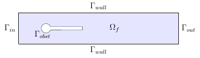
A channel with a cylinder inside

We consider a 2D model representative of a laminar incompressible flow around an obstacle. The flow domain, named $\Omega_f$ , is contained into the rectangle $\lbrack 0,Long \rbrack \times \lbrack 0,Haut \rbrack$ . It is characterised, in particular, by its dynamic viscosity $\mu_f$ and by its density $\rho_f$ .

Geometry of the Turek & Hron HeatFluid Benchmark

TurekHron Geometry

In order to describe the flow, the incompressible Navier-Stokes model is chosen for this case, define by the conservation of momentum equation and the conservation of mass equation. At them, we add the material constitutive equation, that help us to define $\boldsymbol{\sigma}_f$

The goal of this benchmark is to couple the Naviers-Stockes equations and the heat equations We remind that the Naviers-Stokes equation are

$\begin{array}[c]{rl} \rho( \frac{\partial u}{\partial t} + u \cdot \nabla u) - \nu \Delta u + \nabla p & = f\ \mbox{ in } \Omega\\ \nabla \cdot u & = 0\ \mbox{ in } \Omega \end{array}$

And the Heat equations is

$\begin{array}[c]{rl} \rho C_p \left( \frac{\partial T}{\partial t} + \boldsymbol{u} \cdot \nabla T \right) - \nabla \cdot \left( k \nabla T \right) = Q, \quad \text{ in } \Omega \end{array}$

The toolbox is HeatFluid

4. Input parameters

The following table displays the various fixed and variables parameters of this test-case.

Table 1. Fixed and Variable Input Parameters
Name	Description	Units
$u$	fluid velocity	$m/s$
$\rho$	density of the fluid	$kg/m^3$
$\nu$	dynamic viscosity	$kg/(m×s)$
$p$	pression	$Pa$
$f$	source term	$kg/(m^3×s)$
$C_p$	thermal capacity	$J/(kg∗K)$
$T$	Temperature	$K$
$Q$	heat source	$W.m^{-3}$
$k$	Thermal conductivity	$W⋅m^{-1}⋅K^{-1}$

4.1. initial condition

For the fluid:

We use a parabolic velocity profile, in order to describe the flow inlet by $\Gamma_{in}$ , which can be express by

$v_{cst} = 1.5 \bar{U} \frac{4}{0.1681} y \left(0.41-y\right)$

where $\bar{U}$ is the mean inflow velocity.

However, we want to impose a progressive increase of this velocity profile. That’s why we define

$v_{in} = \left\{ \begin{aligned} & v_{cst} \frac{1-\cos\left( \frac{\pi}{2} t \right) }{2} \quad & \text{ if } t < 2 \\ & v_{cst} \quad & \text{ otherwise } \end{aligned} \right.$

With t the time.

For the temperature:

We give as source this temperature

$T_{in}=300*(y>0.15)*(y<0.25)+(293.15*(y<(0.15-1e-9)))+(293.15*(y>(0.25-1e-9)))$

4.2. Materials

    "Materials":
    {
        "Fluid":{
            "rho":"1.0e3",
            "mu":"1.0",
            "k":"2.9e-5",
            "Cp":"4185"
        }
    },

json

4.3. Boundary conditions

For the fluid:

We set

On $\Gamma_{in}$ , an inflow Dirichlet condition : $\boldsymbol{u}_f=(v_{in},0)$
On $\Gamma_{wall}$ and $\Gamma_{obst}$ , a homogeneous Dirichlet condition : $\boldsymbol{u}_f=\boldsymbol{0}$
On $\Gamma_{out}$ , a Neumann condition : $\boldsymbol{\sigma}_f\boldsymbol{ n }_f=\boldsymbol{0}$

For the heat:

On $\Gamma_{in}$ , an inflow Dirichlet condition : $\boldsymbol{T}_f=T_{in}$

4.4. Fields

We are intersting in the visualisation of the three fields : the velocity, the pressure and the temperature of the fluid

            "Exports":
            {
                "fields":["fluid.velocity","fluid.pressure","heat.temperature","fluid.pid"]
            },

4.5. Measures

the pressure is measured on two points to see the behavior of the pressure as a function of time

            "Measures":
            {
                "Forces":"wall2",
                "Points":
                {
                    "pointA":
                    {
                        "coord":"{0.6,0.2,0}",
                        "fields":"pressure"
                    },
                    "pointB":
                    {
                        "coord":"{0.15,0.2,0}",
                        "fields":"pressure"
                    }
                }
            },

json

5. Numerical Experiments

We run this model, using the command labeled at the top, we have the following results.

Temperature:

Velocity

Pressure: