QuarterTurn

In this example, we will estimate the rise in temperature due to Joules losses in a stranded conductor. An electrical potential $V_0$ is applied to the entry/exit of the conductor which is also cooled by a force flow.
The geometry of the conductor is choosen as to have an analytical expression for the temperature.

1. Running the case

The command line to run this case in 2D is

mpirun -np 4 feelpp_toolbox_thermoelectric --case "github:{path:toolboxes/thermoelectric/cases/cvg}" --case.config-file 2d.cfg

mpirun

Case option

--case "github:{path:toolboxes/thermoelectric/cases/cvg}"

Case config file option

--case.config-file 2d.cfg

The command line to run this case in 3D is

mpirun -np 4 feelpp_toolbox_thermoelectric --case "github:{path:toolboxes/thermoelectric/cases/cvg}" --case.config-file 3d.cfg

mpirun

Case option

--case "github:{path:toolboxes/thermoelectric/cases/cvg}"

Case config file option

--case.config-file 3d.cfg

2. Geometry

The conductor consists in a rectangular cross section torus which is somehow "cut" to allow for applying electrical potential. The conductor is cooled with a force flow along its cylindrical faces.+ In 2D, the geometry is as follow:
In 3D, this is the same geometry, but extruded along the z axis.

3. Input parameters

Name	Description	Value	Unit
$r_i$	internal radius	1	$m$
$r_e$	external radius	2	$m$
$\delta$	angle	$\pi/2$	$rad$
$V_D$	electrical potential	9	$V$
$h_i$	internal transfer coefficient	$60e3$	$W\cdot m^{-2}\cdot K^{-1}$
$T_{wi}$	internal water temperature	303	$K$
$h_e$	external transfer coefficient	$58e3$	$W\cdot m^{-2}\cdot K^{-1}$
$T_{we}$	external water temperature	293	$K$

Name

Description

Value

Unit

$r_i$

internal radius

$m$

$r_e$

external radius

$m$

$\delta$

angle

$\pi/2$

$rad$

$V_D$

electrical potential

$V$

$h_i$

internal transfer coefficient

$60e3$

$W\cdot m^{-2}\cdot K^{-1}$

$T_{wi}$

internal water temperature

303

$K$

$h_e$

external transfer coefficient

$58e3$

$W\cdot m^{-2}\cdot K^{-1}$

$T_{we}$

external water temperature

293

$K$

3.1. Model & Toolbox

This problem is fully described by a Thermo-Electric model, namely a poisson equation for the electrical potential $V$ and a standard heat equation for the temperature field $T$ with Joules losses as a source term.
toolbox: thermoelectric

3.2. Materials

Name	Description	Marker	Value	Unit
$\sigma$	electric conductivity	omega	$4.8e7$	$S.m^{-1}$

Name

Description

Marker

Value

Unit

$\sigma$

electric conductivity

omega

$4.8e7$

$S.m^{-1}$

3.3. Boundary conditions

The boundary conditions for the electrical probleme are introduced as simple Dirichlet boundary conditions for the electric potential on the entry/exit of the conductor. For the remaining faces, as no current is flowing througth these faces, we add Homogeneous Neumann conditions.

Marker	Type	Value
V0	Dirichlet	0
V1	Dirichlet	$V_D$
Rint, Rext, top, bottom	Neumann	0

Marker

Type

Value

Dirichlet

$V_D$

Rint, Rext, top*, bottom*

Neumann

As for the heat equation, the forced water cooling is modeled by robin boundary condition with $Tw$ the temperature of the coolant and $h$ an heat exchange coefficient.

Marker	Type	Value
Rint	Robin	$h_i(T-T_{wi})$
Rext	Robin	$h_e(T-T_{we})$
V0, V1, top, bottom	Neumann	0

Marker

Type

Value

Rint

Robin

$h_i(T-T_{wi})$

Rext

Robin

$h_e(T-T_{we})$

V0, V1, top*, bottom*

Neumann

*: only in 3D

4. Outputs

The main fields of concern are the electric potential $V$ , the temperature $T$ and the current density $\mathbf{j}$ or the electric field $\mathbf{E}$ . // presented in the following figure.

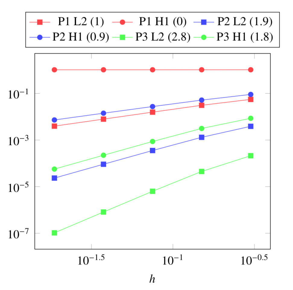
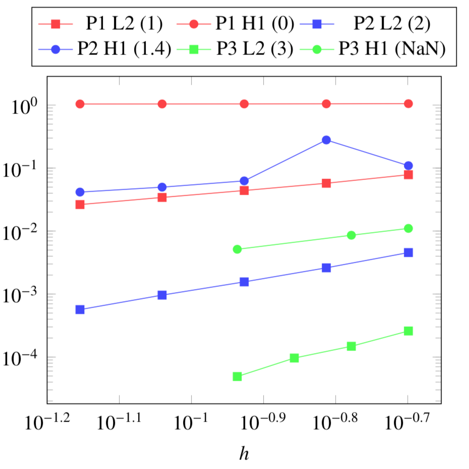
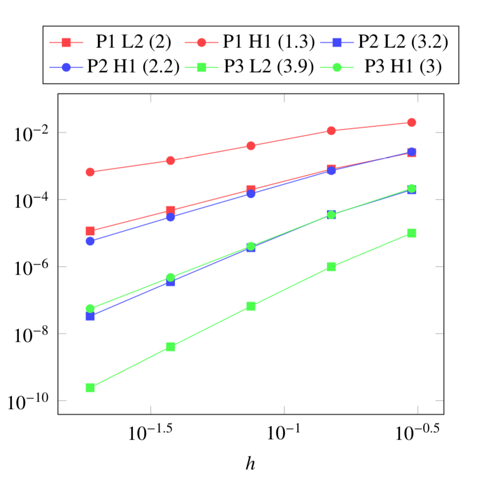
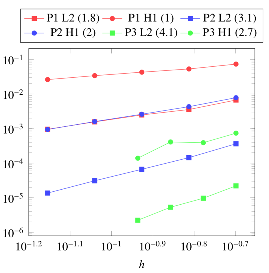
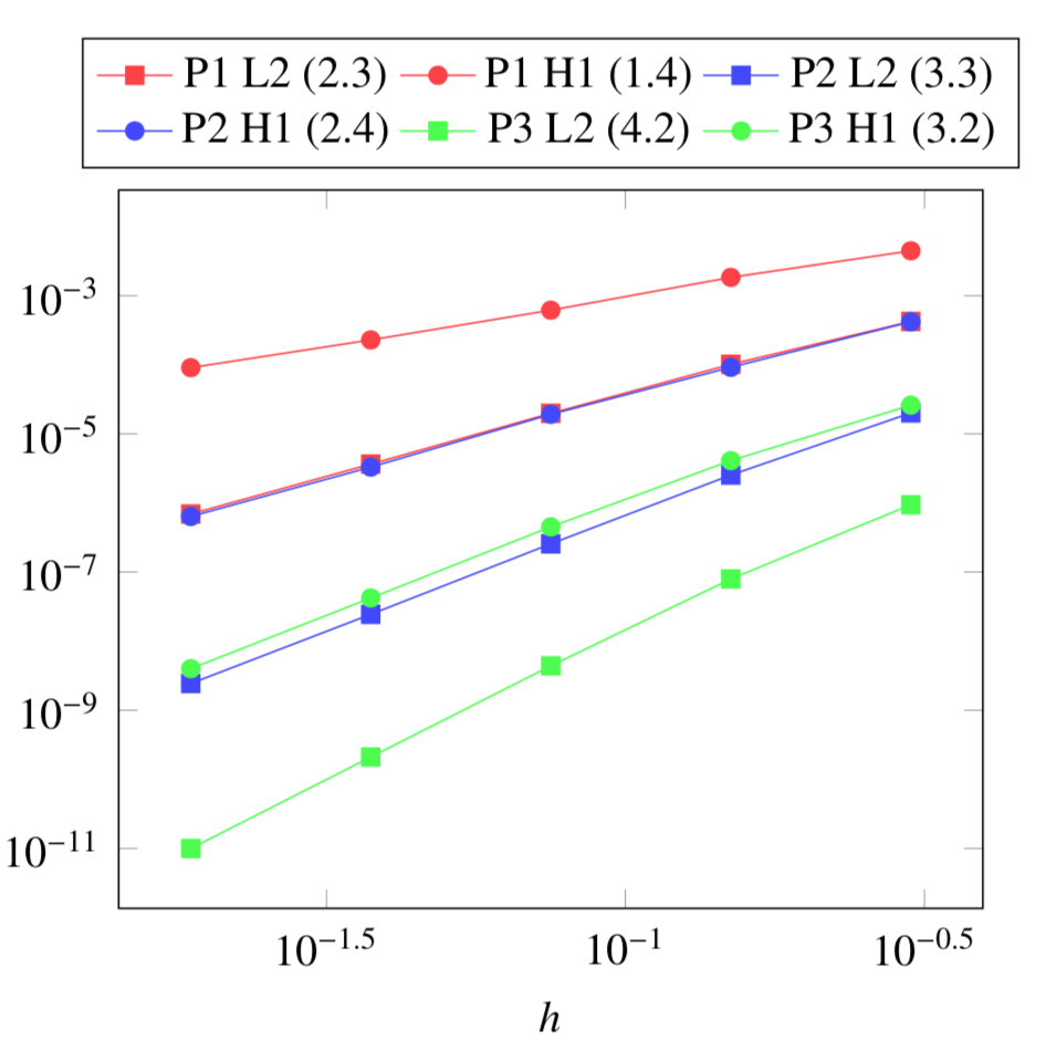
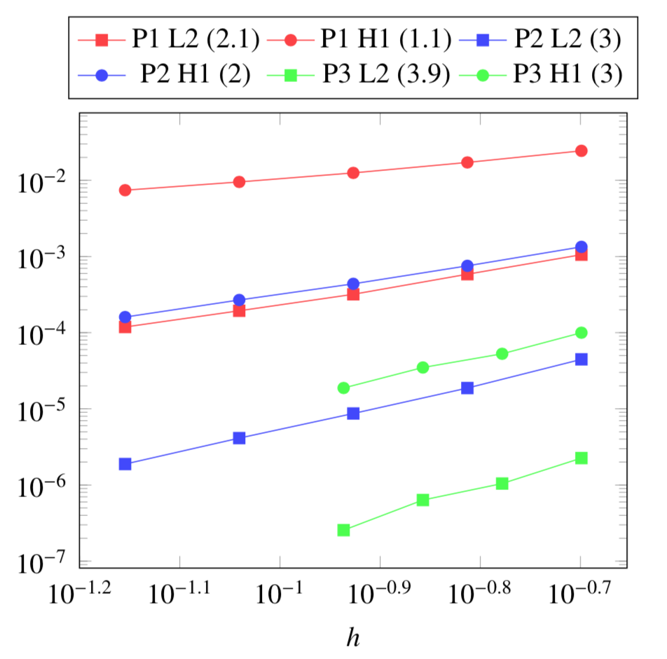
5. Verification Benchmark

The analytical solutions are given by:

$\begin{align*} V&=\frac{V_D}{\delta}\theta=\frac{V_D}{\delta}\operatorname{atan2}(y,x)\\ \mathbf{E}&=\left( -\frac{V_D}{\delta}\frac{y}{x^2+y^2}, \frac{V_D}{\delta}\frac{x}{x^2+y^2}\right)\\ T&=A\log(r)^2+B\log(r)+C=A\log\left(\sqrt{x^2+y^2}\right)^2+B\log\left(\sqrt{x^2+y^2}\right)+C\\ A&=-\frac{\sigma}{2k}\left(\frac{V_D}{\delta}\right)^2\\ B&=\frac{B_e-B_i}{D}\\ C&=\frac{C_e-C_i}{D}\\ B_e&=2T_{we}\delta^2h_eh_ikr_er_i + V_D^2h_eh_ir_er_i\sigma\log(r_e)^2 + V_D^2h_ikr_i\sigma\log(r_e^2)\\ B_i&=2T_{wi}\delta^2h_eh_ikr_er_i + V_D^2h_eh_ir_er_i\sigma\log(r_i)^2 - V_D^2h_ekr_e\sigma\log(r_i^2)\\ C_e&=(h_er_e\log(r_e) + k)(2T_{wi}\delta^2h_ikr_i + V_D^2h_ir_i\sigma\log(r_i)^2 - V_D^2k\sigma\log(r_i^2))\\ C_i&=(h_ir_i\log(r_i) - k)(2T_{we}\delta^2h_ekr_e + V_D^2h_er_e\sigma\log(r_e)^2 + V_D^2k\sigma\log(r_e^2))\\ D&=2\delta^2k(h_eh_ir_er_i\log(r_e) - h_eh_ir_er_i\log(r_i) + h_ekr_e + h_ikr_i) \end{align*}$

We will check if the approximations converge at the appropriate rate:

k+1 for the $L_2$ norm for $V$ and $T$
k for the $H_1$ norm for $V$ and $T$
k for the $L_2$ norm for $\mathbf{E}$ and $\mathbf{j}$
k-1 for the $H_1$ norm for $\mathbf{E}$ and $\mathbf{j}$

Table 1. Temperature 2D and 3D

Table 2. Electric potential 2D and 3D

Table 3. Electric field 2D and 3D