Simulation of a Plateau :: HiFiMagnet Documentation

1. Introduction

Temperature and Magnetic Field profile during experiment

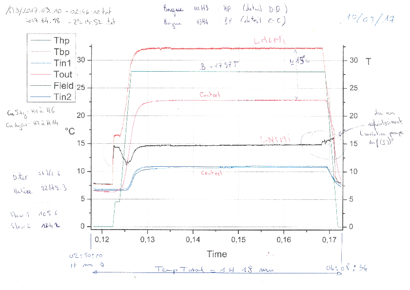
In this example we will try to reproduce the behaviour of an 14 Helices insert operated on March 2017 during a Plateau . More precisely, we will compare:

the voltage tap measurements on HP and BP sides (ie on tap per helix)
the temperature measurement in the rings H2H3 and H3H4.

Beside the HiFiMagnet Salome plugins, the python scripts mentioned in the text may be found here.

2. Input data

Table 1. Electrical Conductivity per helix
Helix	\(\sigma\) [\(M\Omega/m\)]	Nuance
1	52.4	Cu5Ag Cold Spray
2	53.3	"
3	52.6	"
4	52.8	"
5	53.1	"
6	53	"
7	55.6	Cu0.1Ag Cold Spray
8	55.6	"
9	56.1	"
10	55	"
11	55	"
12	55.5	"
13	55.1	"
14	55.4	"

Table 2. Operating conditions
Icoil1 [A]	Tin1 [C]	Tout [C]	HP1 [bar]	BP [bar]	Flow1 [\(l/s\)]	Notes
22148.2	11.0	22.9	14.3	4.0	105.3	use `txt2cvs.py` to view data: eg. `python txt2csv.py --input_file M9_2017.03.10-02_46_10.txt --output_time "03:52:51" --output_key="Icoil1;Tin1;Tout;HP1;BP;Flow1"`

Table 3. Heat exchange coefficients
Model	Notes
Montgomery	see excelsheet `MagnetTools/docs/TemperatureField/Cooling-Coeff.xls` table "14H (version3)"
Others (Colburn,…)	run `NumModel.py` python script with appropriate data from table 2: eg. `python hifimagnet/salome/HIFIMAGNET/src/HIFIMAGNET/NumModel.py Num-HL-31 --geometry HL-31 --CoolantTemp 11 --dT 11.9 --BP 4 --dP 10.3`

For computed heat exchange coefficients, we will select the dataset that gives an estimate flow rate which is the closest to the measured one:

Design value with a constant friction coefficient,
Montgomery with a constant friction coefficient,
Colburn with a constant friction coefficient,
Dittus with a constant friction coefficient,
Silberberg with a constant friction coefficient.

A template thermoelectric model file may be create with:

salome -w1 -t $HIFIMAGNET/HIFIMAGNET_Cmd.py \
  args:--cfg=HL-31.yaml,--setup,--cooling="MeanPressure/DPressure/MeanTemperature",--correlation=colburn,--friction="constant"

with cooling="9.15/10.3/17.4875205"

3. Simulations

Sim

Correlation

Tw

cfg

Cst

cst

Tin1

HL-31_DeMarinis-cst.cfg

Grad

cst

Tw=Tin1+DT1*z

HL-31_DeMarinis.cfg

Mcst

Montgomery

Tin1

HL-31_DeMarinis-montgomery-cst.cfg

Mgrd

""

Tw=Tin1+DT1*z

HL-31_DeMarinis-montgomery-grad.cfg

Cgrd

Colburn

Tw=Tin1+DT1*z

HL-31_DeMarinis-colburn-grad.cfg

Dgrd

Dittus

Tw=Tin1+DT1*z

HL-31_DeMarinis-dittus-grad.cfg

Sgrd

Silberberg

Tw=Tin1+DT1*z

HL-31_DeMarinis-silberberg-grad.cfg

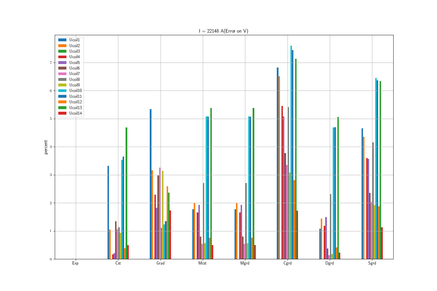
4. Voltage taps

To get the computed voltage taps, we can use:

ensight102 [-X] -batch  -p probe_voltage.py -pyargv -i Electrics.case -o out.data -b -endpyargv
python test.py  --input_file out.data  --exp_file ~/MSO4SC/hifimagnet-msoapps/Examples/HL-31-v105/M9_2017.03.10-02_46_10.txt --bp

To get the measured values:

python txt2csv.py --input_file M9_2017.03.10-02_46_10.txt  --output_time "03:52:51"  --output_key="Ucoil1;...;Ucoil14"

	U1	U2	U3	U4	U5	U6	U7	U8	U9	U10	U11	U12	U13	U14
Exp	6.7	8.1	NA	22.6	13.2	16.0	17.7	20.3	22.9	25.1	27.1	28.6	26.1	24.2
Cst	6.48	8.02	9.99	12.57	13.17	15.79	17.51	20.53	22.69	25.99	28.09	28.49	27.32	24.32
Grad	6.34	7.84	9.78	12.30	12.96	15.52	17.12	20.07	22.18	25.41	27.47	27.86	26.72	23.78
Mcst	6.82	8.26	10.17	12.81	13.45	16.13	17.79	20.85	23.03	26.37	28.47	28.82	27.50	24.32
Mgrd	6.82	8.26	10.17	12.81	13.45	16.13	17.79	20.85	23.03	26.37	28.47	28.82	27.50	24.32
Cgrd	7.16	8.63	10.56	13.28	13.87	16.60	18.29	21.40	23.60	27.01	29.11	29.40	27.96	24.62
Dgrd	6.77	8.22	10.12	12.75	13.40	16.06	17.72	20.77	22.94	26.28	28.37	28.72	27.42	24.25
Sgrd	7.01	8.45	10.36	13.05	13.67	16.38	18.06	21.14	23.34	26.72	28.82	29.14	27.75	24.47

U3 probe was not available. It has been disconnected since it was inducing some problems. As a consequence, U4 actually record the voltage drop between U2 and U4.

Relative error for Voltage taps for each simulation.

5. Temperature probes

To get the computed voltage taps, we can use:

ensight102 [-X] -batch  -p probe_temp.py -pyargv -i Thermics.case -o out.data -b -endpyargv

Obviously, we will only consider simulations where Tw is defined as a gradient for each cooling channel:

	HP [K]	BP [K]
Exp	287.95	305.35
Grad	286.967	294.296
Mgrd	287.052	294.356
Cgrd	287.145	294.413
Dgrd	287.139	294.351
Sgrd	287.101	294.386

6. Helices Mean Temperature

To compute the mean temperature per helix:

ensight102 -X -batch -p $HOME/MSO4SC/hifimagnet-msoapps/Examples/HL-31-v105/view.py -pyargv -i Thermics.case -f T  -endpyargv

The result will be stored in T_vMean.dat.

To get the "measured" values in Celsius:

python txt2csv.py --input_file M9_2017.03.10-02_46_10.txt  --output_time "03:52:51"  --output_key="Tcal1;...;Tcal14"

	T1	T2	T3	T4	T5	T6	T7	T8	T9	T10	T11	T12	T13	T14
Exp	70.3	73.2	NA	74.1	65.5	61.3	63.2	61.2	59.6	57.5	55.6	58.9	46.2	39.2
Cst	46.87	60.77	58.78	57.87	52.32	51.79	49.14	48.59	47.18	46.93	45.52	42.94	39.59	35.61
Grad	38.72	54.01	52.31	51.17	45.98	45.22	42.83	42.06	40.84	40.43	39.21	36.54	33.43	29.48
Mcst	52.00	66.71	61.46	61.15	54.60	54.34	51.28	50.77	49.03	48.81	47.03	43.69	39.35	34.17
Mgrd	49.78	66.25	61.26	60.69	54.40	53.90	51.08	50.33	48.76	48.37	46.76	43.26	39.10	33.75
Cgrd	58.30	77.70	71.00	70.19	62.14	61.38	57.79	56.76	54.72	54.18	52.10	47.89	42.87	36.59
Dgrd	49.07	65.28	60.43	59.88	53.73	53.26	50.50	49.77	48.24	47.87	46.29	42.86	38.77	33.50
Sgrd	54.82	72.41	66.36	65.75	58.59	58.00	54.80	53.94	52.13	51.68	49.83	45.94	41.30	35.36