Magnets Monitoring and Control
1. Magnets Monitoring
In this paragraph we present the main principle of the magnet monitoring.

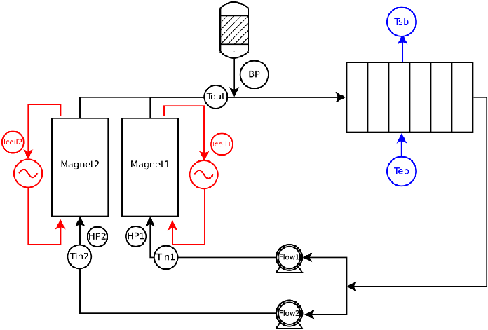
High Field Magnets are electromagnets made of copper alloys tubes - connected into series be so-called ring - powered with up to 31 kA to deliver up to 37 tesla. To dissipate the electric powered the magnet are cooled by a water forced flow (up to 140 l:m³ with a pressure drop of 25 bars). Therefore the magnets are actually set into a housing. Such environment (water and high pressure) make it difficult to instrument the magnets.
The only available measures come from:
-
voltage taps on the connection ring between consecutive tube,
-
water temperature probes at the inlet and outlet of the cooling circuit,
-
flow rate sensor.
In addition to these data, we also have access to:
-
the total voltage drop \(V\),
-
the total electric power \(P\),
-
and the field factor \(f\), ie. the ratio of the magnetic field \(B_z(0)\) at the magnetic center over the input current \(I\). \(f\) is experimentally obtained by measuring the magnetic field profile along the magnet \(Oz\) axis at a given current. Note that this actually relies on the hypothesis of linear dependency of \(ß\) versus \(I\).
The magnet is actually operated by setting the input current \(I\). In practice, the user request a value of \(B_z(0)\) on a console which, in turn, send an order to power supply to deliver a current \(I=\frac{B_z(0)}{f}\). During this operation, the monitoring system receive data from the voltage taps \(U_i\), water temperatures probes (\(Ti, To\)) and flow rate \(Q\) sensor.
In this example, the magnet consists in 2 "tranches" operating at 9h57 and providing a 18.8 tesla magnetic field:
Coils 1 to 7 correspond to the PolyHelix insert (one per couple of helices); Coils 15 and 16 to the Bitters. Data specific to each "tranche" is appended with the tranche index. \(dPm1\) denote the pressure drop from HP and BP side on tranche 1 where HP, BP stand respectively for High and Low ("Basse" in french) Pressure. \(T_i\) denote the estimated mean temperature in Coil \(i\). See bellow for more details. |
Actual data from an magnet in operation may be retreive from the control/command monitoring system at an acquisition rate of 1 Hz. This site, ony accesible to registered {lncmi} user, provides data recorded during a magnet run. To access a magnet run:
-
Go to the menu Courbes/Fichier Aimants.
-
Select a file
txtfrom a site (eg M9).
You can then explore the magnet data and download the file for latter use by clicking on Télécharger txt.
The txt file may be converted to a csv file using txt2cvs.py. An example can be found here.
There are also files with an higher acquisation rate available. They may be used as refrence for transient analysis.
Data from these tdms file can be retreived using nptdms-ex.py script.
2. Magnets Control
The control system relies on these data to determine if the operating magnet is safe or not. More precisely it checks the deviation \(dR0_i\) of the resistance measured for each voltage tap (ie \(R0_i = \frac{U_i}{I}\)) from a reference value. An heuristic threshold of 3% is considered as an indicator of a wrong behavior. Once this threshold is reached, a signal is send to power supply leading to a controlled power shutdown. This means that \(I\) is driven to 0 in a controlled manner (typically in roughly a tenth of second).
The reference values for \(R0_i\) are determined during the magnet commissioning following this process:
-
For \(I_n\)
-
Measure \(U\) per helix (or couple of helices)
-
Compute \(R=\frac{U}{I}\)
-
Repeat for new \(I_n+1\) until 30 kA is reached
Then, a fit for each \(R\) as a 2nd order polynomial of \(I\) is computed. This fit will also be usefull to have an estimate of the mean temperature \(<T>\) of the helix (or couple of helices):
with \(T_0\) a reference temperature (generally 20C).
|
-
ToDo:
-
Add note on Control/Command website
-
Add note on txt files (with a demo)
-