 .pdf
.pdf
Boustrophedon Cellular Decomposition
1. Introduction
The Boustrophedon Cell Decomposition (BCD) is a method for coverage path planning for cleaning robots.
This cell decomposition method divides the robot’s reachable area into non-overlapping cellular regions.
The robot’s trajectory is then determined by the sequence of cells to be visited.
2. Boustrophedon motion algorithm :
2.1. Description of the Boustrophedon motion algorithm
The different steps of the algorithm simulating the boustrophedon movement of a robot in a rectangular area are given by :
-
Initialization: The algorithm begins by initializing the variables that will be used to track the robot’s movement. The
xandycoordinates are set to zero to indicate that the robot starts at the origin. Timetimeis also initialized to zero. Velocity variablesvelocity_x,velocity_y, andvelocityare initialized to zero, as the robot is not moving at the start. -
Input parameters: Input parameters are defined, such as the height
heightand widthwidthof the rectangular area in which the robot is placed, the radiusradiusof the robot, the spacedeltabetween the robot and the boundary of the domain, the horizontalstep_Hand verticalstep_Vdisplacement steps, and the time stepdt. -
Displacement computation: The variables
deplacement_Handdeplacement_Vare computed using the robot’s radius, horizontal and vertical displacement steps.deplacement_Hrepresents the distance covered horizontally by the robot during each iteration, whiledeplacement_Vrepresents the distance covered vertically. -
Boustrophedon movement: A
whileloop is used to perform the boustrophedon movement. The robot continues to move as long as its(x, y)coordinates do not exceed the limits of the domain defined byheightandwidth. -
Control variable
move: Themovevariable is used to track the current stage of the boustrophedon movement. It takes values from 0 to 3, where each value represents a direction of movement. The robot performs alternating horizontal and vertical movements according to the value ofmove. -
Horizontal and vertical movements: Depending on the value of
move, the robot performs horizontal and vertical movements, advancing by one step at each iteration. The robot coordinates(x, y)are updated according tostep_Horstep_V. -
Velocity calculation: At each iteration, the velocities
velocity_xandvelocity_yare computed using the movement step and the time stepdt. The total velocityvelocitycorresponds to the Euclidean norm. -
Saving data: At each iteration, the coordinates and velocities are saved in the two lists
cellsandcells_velocityrespectively. Once the boustrophedon movement has been completed, these lists are used to save the data in CSV filesposition.csvandvelocity.csv. -
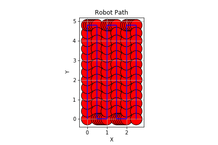
Path visualization: Finally, the path traveled by the robot is visualized using the coordinates stored in
position.csv. The robot is represented by red circles and the path is drawn in blue.
2.2. Boustrophedon motion algorithm :
The Boustrophedon motion algorithm simulates the motion of a robot in a given rectangular area, and records the robot’s coordinates and velocities at each iteration.
Input parameters :
-
heightandwidth: The height and width of the rectangular area. -
radius: Radius of the robot. -
delta: Space to avoid that the robot touches the boundary of the area. -
step_Handstep_V: Horizontal and vertical displacement steps.
Variables:
-
xandy: Position of the robot. -
time: Current simulation time. -
velocity_xandvelocity_y: Robot velocity in x direction and y direction. -
velocity: Total robot velocity. -
cells: List of coordinates (x, y). -
cells_velocity: List of velocities (velocity_x, velocity_y).
Displacement computation:
-
displacement_H: Horizontal displacement computed by dividing twice the robot radius by the horizontal step (step_H). -
displacement_V: Vertical displacement calculated by dividing the total height by the vertical step (step_V).
Control variable:
-
move: Control variable used to track the stage of boustrophedon movement. It takes values from 0 to 3, where each value represents a direction of movement:-
move = 0: Robot moves vertically upwards. -
move = 1ormove = 3: The robot moves horizontally to the right. -
move = 2: The robot moves vertically downwards.
-
Velocity computation:
-
Velocity_xis given by \(v_x = \frac{\Delta x }{ \Delta t}\). -
Velocity_yis calculated as \(v_y = \frac{\Delta y}{\Delta t}\). -
Total
velocityis calculated using the Euclidean norm: \(v = \sqrt{v_x^2 + v_y^2}\).
Boustrophedon motion loop:
Boustrophedon movement is performed using a while loop, which continues as long as the robot is within the zone defined by the dimensions height and width.
The implementation is given by:
def generate_file_csv(height, width, radius, delta, step_H, step_V, time, dt):
    delta_x = step_H # horizontal step
    delta_y = step_V # vertical step
    H = height
    W = width
    cells = [] # list of positions
    x = 0
    y = 0
    time = 0
    cells_velocity = [] # list of velocities


    cells.append([x, y, time]) # add the first cell
    move = 0

    deplacement_H = (2 * radius) / (delta_x) # horizontal displacement
    deplacement_V = height / (delta_y) # vertical displacement

    while ((y + 2*radius + delta) < H and (x + 2*radius + delta) < W): # while the robot remains in the domain

        if move == 0 :
            for i in range(int(deplacement_V - radius - delta)): # vertical displacement
                x = x
                y += delta_y
                cells.append([x, y, time])
                time += dt

                velocity_x = 0 # horizontal velocity
                velocity_y = delta_y / dt # vertical velocity
                velocity = np.sqrt(velocity_x**2 + velocity_y**2) # velocity
                cells_velocity.append([velocity_x, velocity_y, time]) # add velocity to the list

            move = move + 1

        if (move == 1) or (move == 3) :
            for i in range(int(deplacement_H - delta)):  # horizontal displacement
                x += delta_x
                y = y
                cells.append([x, y, time])
                time += dt

                velocity_x = delta_x / dt
                velocity_y = 0
                velocity = np.sqrt(velocity_x**2 + velocity_y**2)
                cells_velocity.append([velocity_x, velocity_y, time])

            move = move + 1 # next move

        if move == 2 :
            for i in range(int(deplacement_V  - radius - delta)):
                x = x
                y -= delta_y
                cells.append([x, y, time])
                time += dt

                velocity_x = 0
                velocity_y = - delta_y / dt
                velocity = np.sqrt(velocity_x**2 + velocity_y**2)
                cells_velocity.append([velocity_x, velocity_y, time])

            move = move + 1

        move = move % 4 # reset move
3. Results
To visualize the robot’s trajectory, we read the csv file of positions (which contains x, y cells and time), create cells covering the entire domain and make the robot follow the path created. In this way, we can have different horizontal and vertical steps.
In our case, we have the following input parameters:
-
height = 5
-
width = 3
-
radius = 0.3
-
delta = 0.1
Vertical and horizontal displacements are respectively given by : step_V = 0.4 and step_H = 0.1.
This gives the following result:
To simulate the robot’s trajectory in a fluid, we use the fluid toolbox of the Feel++ finite element library
and the csv file containing the velocities.
And here we have the visualization of the robot’s trajectory to traverse the given domain on Paraview.
4. Conclusion
In this chapter, we presented the Boustrophedon cell decomposition algorithm, a method for solving the coverage trajectory planning problem for cleaning robots in a given domain. We implemented this algorithm using Python and simulated the robot’s trajectory in a fluid domain using Feel++.