 .pdf
.pdf
Two Dimensional Three Sphere Swimmer
In this example, we want to check if the 2D-three sphere swimmer can present a self propulsion using the same strategy of swimming proposed by Najafi and Golestanian in their paper BCGP2020. This model can be used to show the efficiency of reinforcement learning of swimmers as the 2D simulations are less expensive in terms of iterations and time, especially with an increased number of spheres.
1. 2D-Three sphere swimmer
The 2D-three sphere swimmer is composed of three circles of radius \(R\) linked by two rigid arms of length \(d\) that can change.
As the 3D case, for this model, there is only one non-reciprocal periodic strategy of swimming proposed by Najafi and Golestanian in the figure below :
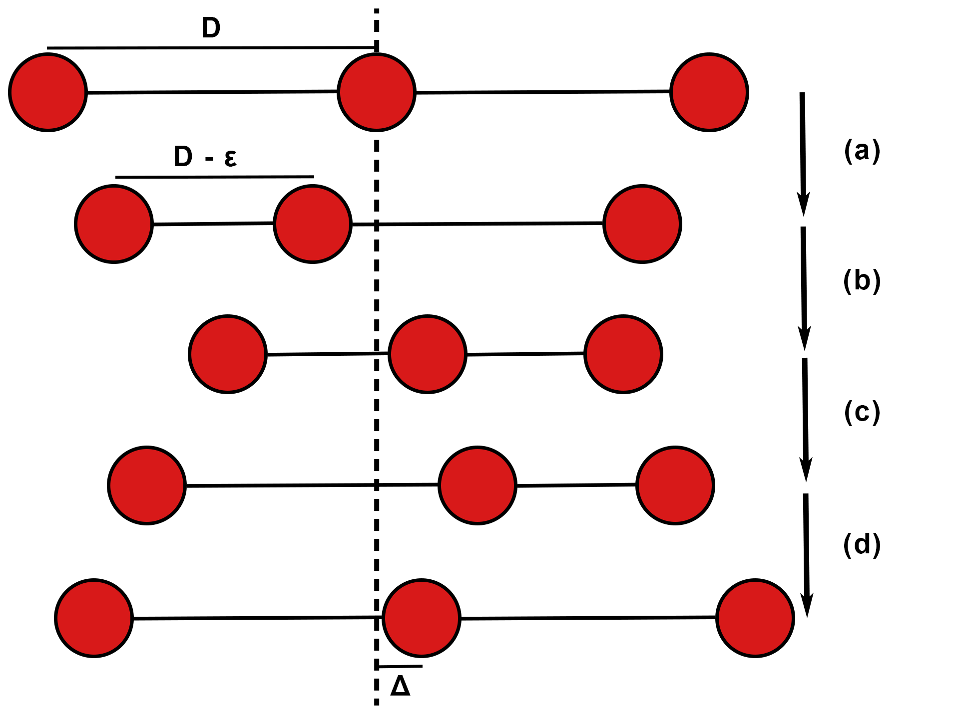
The cycle consists of four consecutive strokes :
-
a) The left arm decreases its length.
-
b) The right arm decreases its length with the same velocity.
-
c) The left arm opens up to its original length.
-
d) The right arm elongates to its original size.
The relative velocity when retracting and elongating at these four strokes is the same.
2. Geometry
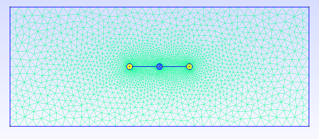
The swimmer described above, is places at the center of a 2D rectangular channel of dimension \([-L,L]\times [-l,l]\). The figure below shows the geometry with meshing :
3. Inpute parameters
Name |
Description |
values |
Unit |
\(R\) |
spheres raduis |
1 |
\(\mu m\) |
\(D\) |
arm length |
\(10R\) |
\(\mu m\) |
\(\varepsilon\) |
relative displacement of the spheres |
\(4R\) |
\(\mu m\) |
\(L\) |
length parameter |
50 |
\(\mu m\) |
\(l\) |
width parameter |
20 |
\(\mu m\) |
4. Materials
Name |
Description |
values |
Unit |
\(\rho_{fluid}\) |
fluid density |
1 |
\(kg/m^3\) |
\(\rho_{spheres}\) |
spheres density |
0.1 |
\(kg/m^3\) |
\(\mu\) |
viscosity |
1 |
\(N.s/m^2\) |
5. Run simulations
The command line to run the simulations is :
mpirun -np 4 feelpp_toolbox_fluid --config-file three_sphere_2D.cfg6. Results
6.1. Analytical results
Unlike the 3D three-sphere swimmer studied by Najafi and Golestanian in their article, there are no analytical results yet about the displacement quantity for this two -dimensional model. But there will be, for sure, a net displacement at the and of each period since the constraints of the scallop theorem are escaped.
6.2. Numerical results
Here, using the fluid toolbox, we check if the swimmer presents a self-propulsion as expected. The displacement of the center sphere is shown in the figure below :
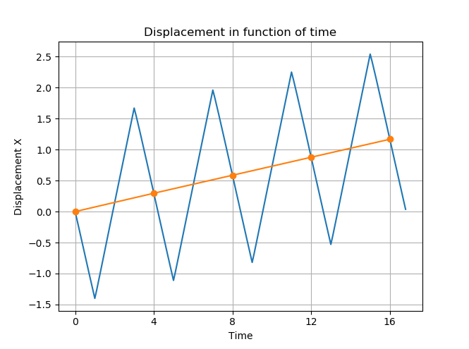
The figure above shows in blue the displacement of the 2D swimmer for \(T_{final} =20s\). The orange line intersects the trajectory of the central sphere at orange circles. The net displacement obtained at each period is equal to 0.29 (for \(R=1\)).
6.3. Comparaison between 2D and 3D cases
Here, we compare our numerical results for the 2D sphere swimmer with the results given in Berti’s paper [bgp_cemracs_2019] for the 3D swimmer.
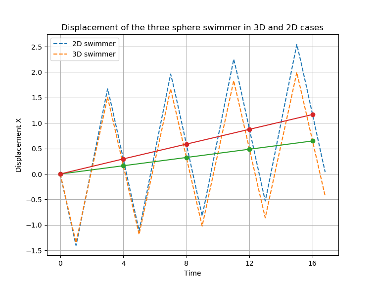
The figure shows the displacement for the 2D and 3D swimmers. orange dashed line represents the displacement of the 3D swimmer given in Berti’s paper and the blue dashed one represents the displacement of the 2D swimmer we found. The red and green lines intersect the trajectories of the central spheres of the 2D and 3D swimmers (respectively) at the red and green circles (respectively).
As a comparison between the 2D and 3D cases, we can see that the results are qualitatively the same while they are not quantitatively. The net displacements of the swimmer in the 2D and 3D cases after finishing a periodic cycle are given as follow :
-
2D swimmer achieve a net displacement equal to 0.30.
-
3D swimmer achieve a net displacement equal to 0.16.
References on Swimming
-
[Najafi_2004] Ali Najafi, Ramin Golestanian. Simple swimmer at low Reynolds number: Three linked spheres. 2004. American Physical Society. doi.org/10.1103/PhysRevE.69.062901 linkDownload PDF
-
[nature] Jikeli, J., Alvarez, L., Friedrich, B. et al. Sperm navigation along helical paths in 3D chemoattractant landscapes. Nat Commun 6, 7985 (2015). doi.org/10.1038/ncomms8985 Download PDF
-
[bgp_cemracs_2019] Luca Berti, Laetitia Giraldi, Christophe Prud’Homme. Swimming at Low Reynolds Number. ESAIM: Proceedings and Surveys, EDP Sciences, 2019, pp.1 - 10, doi.org/10.1051/proc/202067004 Download PDF
-
[bcgp_three_spheres_2020] Luca Berti, Vincent Chabannes, Laetitia Giraldi, Christophe Prud’Homme. Modeling and finite element simulation of multi-sphere swimmers. 2020. hal-mines-paristech.archives-ouvertes.fr/ENSMP_CEMEF/hal-03023318v1 Download PDF
-
[gbcc_epje_2017] K. Gustavsson, L. Biferale, A. Celani, S. Colabrese Finding Efficient Swimming Strategies in a Three Dimensional Chaotic Flow by Reinforcement Learning Published on Eur. Phys. J. E (December 14, 2017) 10.1140/epje/i2017-11602-9 Download PDF
-
[purcell_1977] E.M. Purcell. Life at Low Reynolds Number, American Journal of Physics vol 45, p. 3-11 (1977). doi.org/10.1119/1.10903 Download PDF