 .pdf
.pdf
Design of experiments
1. Description
In this example, we study the 2D-three sphere swimmer with different values of the following parameters :
-
\(y\) : the Y-axis initial position of the swimmer
-
\(R\) : the sphere raduis
-
\(L\) : the lenght of arms
The parameters above can take values in the intervals shown in the following table :
Parameter |
interval |
\(y\) |
[0, 18] |
\(R\) |
[ \(\frac{1}{2}\), \(\frac{3}{2}\)] |
\(L\) |
[10, 14] |
We want to perform twenty different simulations for different values of the parameters above. For that, we use the Latin Hypercube Sampling method (LHS) as the obtained points can be spread out in such a way that each dimension is explored.
2. Latin Hypercube Sampling method
2.1. LHS
The LHS design is a simple high dimensional statistical method that generates quasi-random sampling distributions. The method works as follow : each dimension space representing a variable is cut into \(n\) sections (\(n\) is the number of the sampling points) and only one point is put in each section. For more details about the LHS method, see [Add a link here]
2.2. Usage
The LHS design is defined in many python libraries such as scipy, openturns, smt, … Here, we give a simple example using LHS method with smt python library.
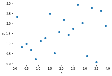
The code below generates twenty samples in the interval \([0, 4]\times[0, 3]\) with the LHS method.
import numpy as np
import matplotlib.pyplot as plt
from smt.sampling_methods import LHS

xlimits = np.array([[0, 4], [0, 3]])
sampling = LHS(xlimits=xlimits)

num = 20
x = sampling(num)
plt.plot(x[:, 0], x[:, 1], "o")
plt.xlabel("x")
plt.ylabel("y")
plt.show()
The figure below, shows the samples chosen with LHS method in the interval \([0, 4]\times[0, 3]\).
2.3. Application to our model
In our case, as we want to perform twenty simulations (samples) and we have three parameters, the domain where the samples are generated is \([0, 18]\times [0.5, 1.5]\times [10, 14]\). Here is the code in python.
import numpy as np
import matplotlib.pyplot as plt
from smt.sampling_methods import LHS

xlimits = np.array([[0, 18], [0.5, 1.5], [10, 14]])
sampling = LHS(xlimits=xlimits)

num = 20
x = sampling(num)
plt.plot(x[:, 0], x[:, 1], "o")
plt.xlabel("x")
plt.ylabel("y")
plt.show()