PMPY Swimmer

In this example, we simulate the pushemepullyou swimmer in 2D and 3D using the \(Feel\)++ fluid toolbox. Then, we compare our results with the theoretical ones provided for the 3D model in [Avron_pmpu].

1. PMPY swimmer

1.1. 3D model

As described in [Avron_pmpu], the pushmepullyou swimmer consists of two elastic spheres that can exchange volumes. These two spheres are attached by a rigid arm that can change its length. Since this model has two degrees of freedom, it can perform many different non-reciprocal strokes that guarantee the self-propulsion of the swimmer.

A simple non-reciprocal motion was presented in [Avron_pmpu] as follow

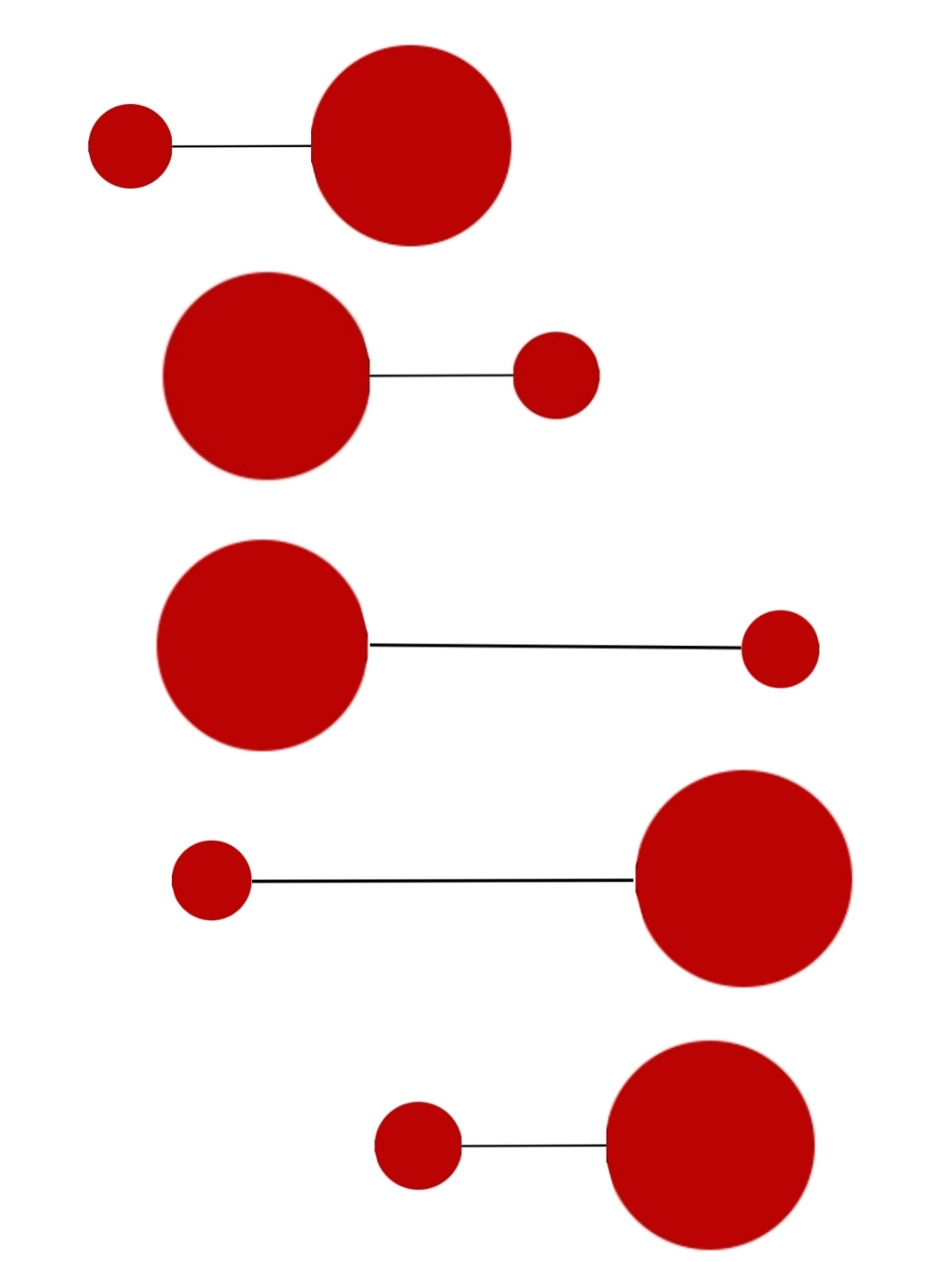
We note that the total volume of the spheres is conserved during this cyclic motion.

1.2. 2D model

The two-dimenssional model consists of two disks instead of spheres. The disks can exchange surfaces such that the total surface of the two disks is conserved.

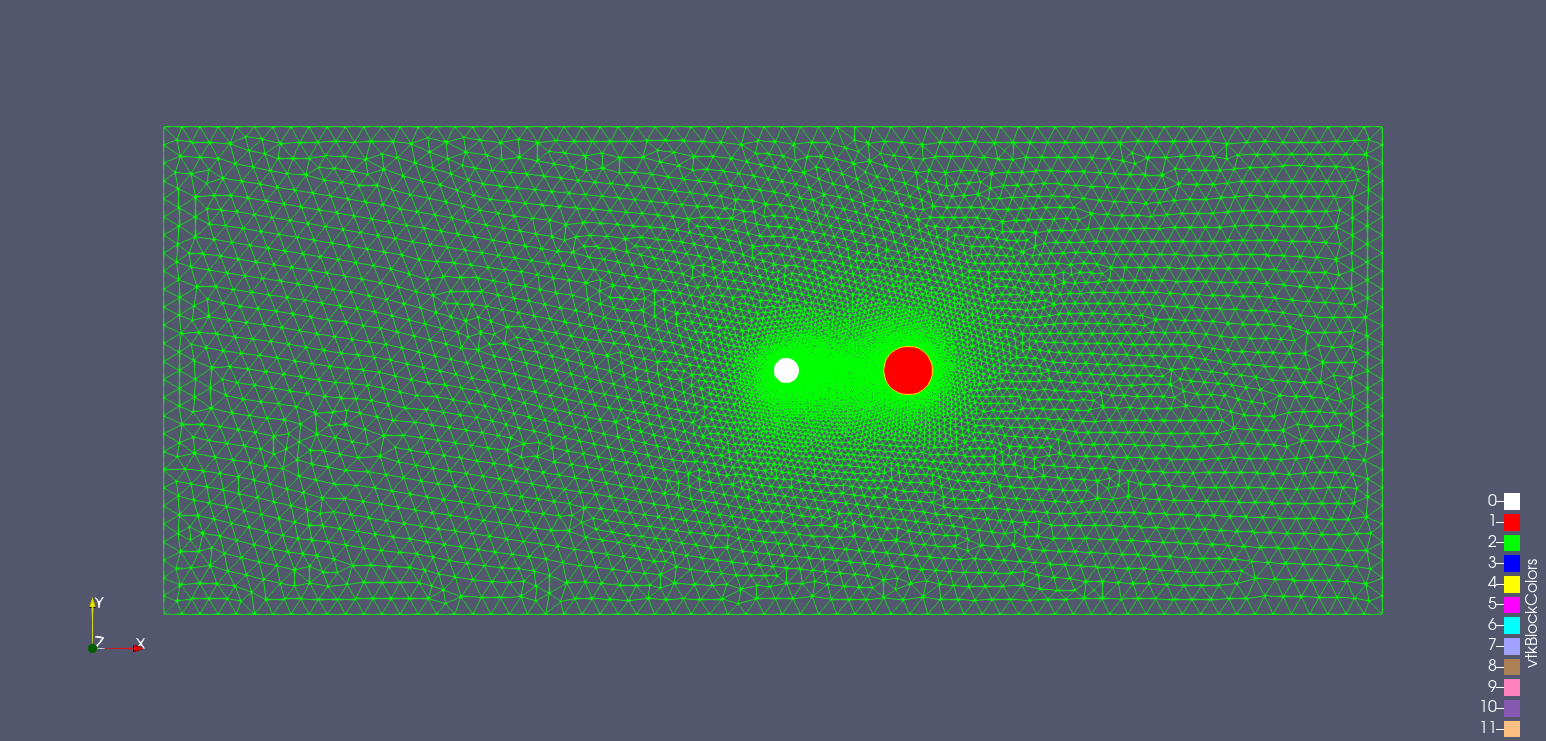
2. Geometry & Mesh

2.1. 2D model

The geometry consists of a rectangular channel of dimensions \([-l_1,l_1]\times [-l_2,l_2]\). The swimmer is placed in the middle of the channel as can be seen in the figure below. Note that, for conserving the total surface of the two disks, they should have the same number of mesh elements (triangles).

2.2. 3D model

In 3D, it is the same geometry, but the chennel is extruded along the z axis and the disks are replaced by spheres. The channel occupies the domain \([-l_1,l_1]\times [-l_2,l_2]\times [-l_3,l_3]\).

Again, while meshing the 3D geometry, the spheres should have the same number of tetrahedrons for the conservation of the total volume.

3. Inpute parameters

Name

Description

values

\(a_{min}\)

left sphere raduis

\(a_{max}\)

right sphere raduis

\(L\)

arm length

\(10\)

\(\varepsilon\)

relative displacement of the spheres

\(4\)

\(l_1\)

length parameter

\(l_2\)

width parameter

\(l_3\)

height parameter

4. Materials & Boundary conditions

4.1. Materials

Name

Description

values

Unit

\(\rho_{fluid}\)

fluid density

\(kg/m^3\)

\(\rho_{spheres}\)

spheres density

0.1

\(kg/m^3\)

\(\mu\)

viscosity

\(N.s/m^2\)

4.2. Boundary conditions

For the 2D model, We imposed a homogenous Dirichlet condition on the top and bottom walls and a Neumann condition on the left and right walls

Marker

Interval

Type

Value

top wall, bottom wall

\([-l_1,l_1]\times \{-l_2,l_2\}\)

Dirichlet

\((0,0)\)

left wall, right wall

\(\{-l_1,l_1\}\times [-l_2,l_2]\)

Neumann

\(0\)

For the 3D model, we imposed a Neumann condition on the left and right walls. For the other faces, we imposed a Dirichlet condition on the fluid velocity.

Marker

Interval

Type

Value

left wall, right wall

\(\Gamma_1\)

Neumann

\(0\)

top, bottom, front, back walls

\(\Gamma_2\)

Dirichlet

\((0,0,0)\)

where :

\(\Gamma_1\) = \(\{-l_1,l_1\}\times [-l_2,l_2]\times [-l_3,l_3]\)
\(\Gamma_2\) = \(\displaystyle{[-l_1,l_1]\times [-l_2,l_2]\times \{-l_3,l_3\} \bigcup\; [-l_1,l_1]\times \{-l_2,l_2\}\times [-l_3,l_3]}\)

5. Results & Verification Benchmark

5.1. Analytical results

For small deformations, the net displacement of the 3D PMPY swimmer after completing one cycle is given in [Avron_pmpu] as

\[\Delta = \left(\frac{a_{max}-a_{min}}{a_{max}+a_{min}}\right) (\ell_{max}-\ell_{min}).\]

We note that \(\displaystyle{\Delta = \frac{dx_l+dx_r}{2}},\) where \(x_l\) and \(x_r\) denote the center of mass of the left and the right spheres (disks in 2D case) respectively.

In our case, we have :

\(a_{min}\) : radius of the left sphere
\(a_{max}\) : radius of the right sphere
\(\ell_{min} = L\)
\(\ell_{max} = L+\varepsilon\)

5.2. Numerical experiment

In our case, we set the following parameters for both 2D and 3D models

\(a_{min} = 1\)
\(a_{max} = 2\)
\(\ell_{min} = L = 10\)
\(\ell_{max} = L+\varepsilon = 14\)

Let \(r\) and \(R\) be the radii of the left and the right spheres (disks for 2D model) respectively. Let \(T=4s\) be the period of the cyclic motion mentioned above. Each stroke of the motion is performed in \(\frac{T}{4}=1s\).

In our simulations (both 2D and 3D), \(r\) is given by

\[ r(t) =\begin{cases} a_{min}+sin(\frac{\pi}{2}t) & \text{if } t\in[0,1],\\ a_{max} & \text{if } t\in[1,2],\\ a_{max}+sin(\frac{\pi}{2}t) & \text{if } t\in[2,3],\\ a_{min} & \text{if } t\in[3,4]. \end{cases} \]

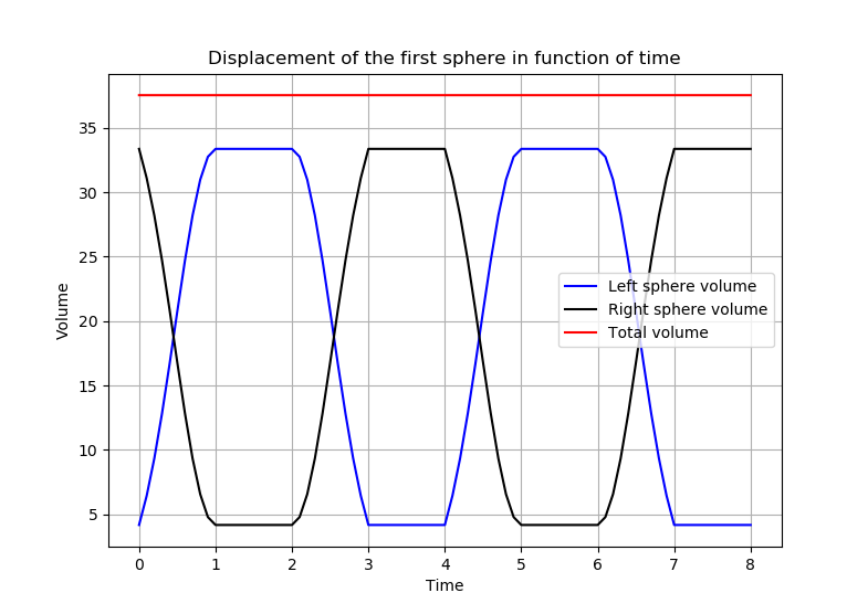
We note that \(R\) is changing in such a way that guarantees the conservation of the total volume (total surface in 2D).

For the two-dimensional model, \( R\) takes the form :

\[ R(t) = \sqrt{a_{min}^2 + a_{max}^2 - r(t)^2}. \]

In \(3D, R\) is given by

\[ R(t) = \sqrt[3]{a_{min}^3 + a_{max}^3 - r(t)^3}. \]

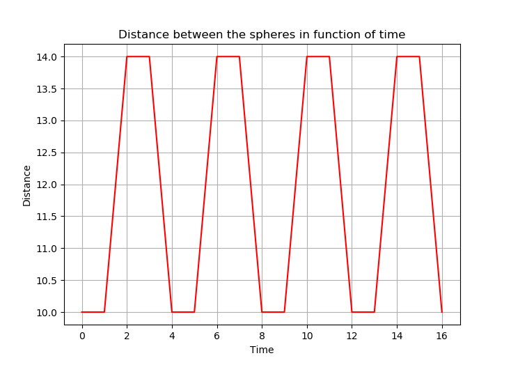
5.3. Results

5.3.1. 2D model

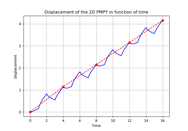
We ran our simulation for \(T_{final}=16s\).

The surfaces of the two disks are changing as follow :

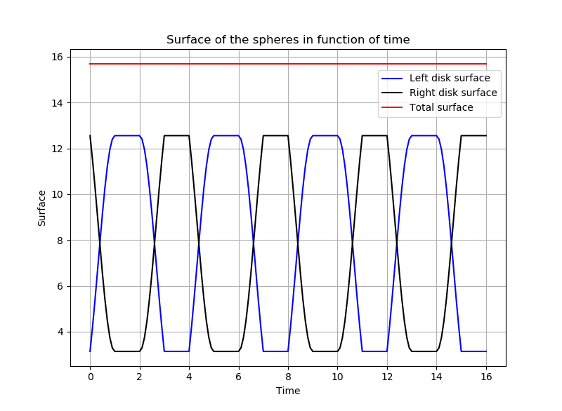
The length of the arm during the four cycles is shown in the figure below

The displacement of the swimmer

5.3.2. 3D model

We ran the simulation for \(T_{final}=8s\).

The volumes of the two spheres are conserved along the 4-strokes as shown in the figure below :

Here we present the displacement of the swimmer in function of time.

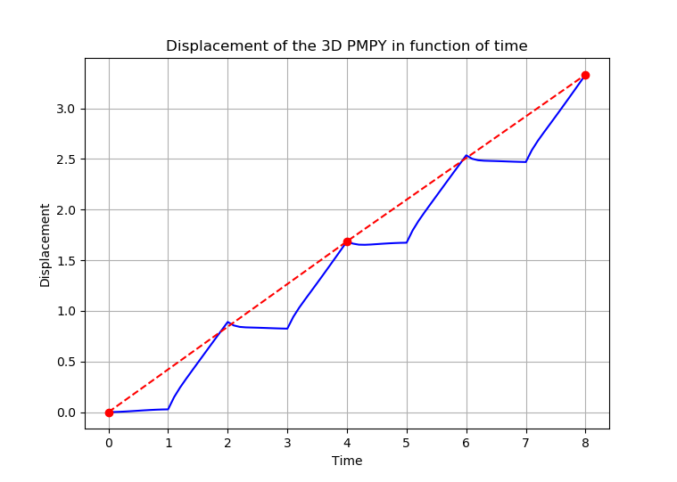
At the end of one periodic cycle, the swimmer is displaced by \(1.68\), while the theoretical net-displacement base on [Averon_pmpu] is \(1.33\).

We note that the theoretical displacement is given under the following assumptions :

\[\frac{a_i}{\ell}\ll 1\qquad\text{and}\qquad a_{min}\ll a_{max}, \]

where \(a_i\) stands for the radii of the two spheres and \(\ell\) denotes the distance between the spheres.

6. Methodology

6.1. Running the simulation

Here is the command line to run the python script that runs the simulation.

mpirun -np 10 python3 fluid-remesh.py

6.2. Json file

Here we present some important sections of the \(json\) file we used to simulate the 2D model with \(PyFeel++\).

We start with specifying the equations describing our model in the \(json\) file as follow.

"Models":
    {
        "equations":"Stokes"
    },

The materials parameters are defined in this section.

"Materials":
    {
        "Fluid":{
            "physics":"fluid",
            "rho":"1",
            "mu":"1"
        },
        "CirLeft":{
            "physics":"body",
            "rho":1e-1
        },
        "CirRight":{
            "physics":"body",
            "rho":1e-1
        }
    },

Here, we specified some parameters that we use to compute the elastic displacement of the spheres.

"Parameters":
    {
        "eps":1e-10,
        "ref_radius_disk_right":2,
        "ref_radius_disk_left":1,
        "radius_left_new":2,
        "diff_left_radii":"(radius_left_new-ref_radius_disk_left):radius_left_new:ref_radius_disk_left",
        "total_radii":"ref_radius_disk_right^2+ref_radius_disk_left^2:ref_radius_disk_right:ref_radius_disk_left",
        "distance_center_right":"max(sqrt((x-10)^2+(y-0)^2),1e-12):x:y",
        "distance_center_left":"max(sqrt((x-0)^2+(y-0)^2),1e-12):x:y",
        "disp_magnitude_left":"diff_left_radii*(sin(pi*t/2)*(pulse(t,0,1-eps,4)+pulse(t,1-eps,1,4))+pulse(t,1,2,4)+sin(pi*t/2-pi/2)*pulse(t,2,3,4)+0*(pulse(t,3,4-eps,4)+pulse(t,4-eps,4,4)))*distance_center_left/ref_radius_disk_left:t:eps:distance_center_left:diff_left_radii:ref_radius_disk_left",
        "disp_magnitude_right":"((sqrt(total_radii-(1+diff_left_radii*sin(pi*t/2))^2)-2)*(pulse(t,0,1-eps,4)+pulse(t,1-eps,1,4))-(ref_radius_disk_right-sqrt(total_radii-radius_left_new^2))*pulse(t,1,2,4)+(sqrt(total_radii-(1+diff_left_radii*sin(pi*t/2-pi/2))^2)-2)*pulse(t,2,3,4)+0*(pulse(t,3,4-eps,4)+pulse(t,4-eps,4,4)))*distance_center_right/ref_radius_disk_right:t:eps:distance_center_right:ref_radius_disk_right:radius_left_new:total_radii:diff_left_radii",
        "disp_vector_normalized_left":"{(x-0)/distance_center_left,(y-0)/distance_center_left}:x:y:distance_center_left",
        "disp_vector_normalized_right":"{(x-10)/distance_center_right,(y-0)/distance_center_right}:x:y:distance_center_right"
    },

In this section we specified the boundary conditions including the elastic and the relative displacements of the two spheres.

"BoundaryConditions":
    {
        "velocity":
        {
            "Dirichlet":
            {
                "BoxWallsDir":
                {
                    "expr":"{0,0}"
                }
            }
        },
        "fluid":
        {
            "outlet":
            {
                "BoxWallsNeu":
                {
                    "expr":"{0}"
                }
            },
            "body":
            {
                "CircleRight":
                {
                    "markers":["CircleRight"],
                    "materials":
                    {
                        "names":["CirRight"]
                    },
                    "articulation":
                    {
                        "body":"CircleLeft",
                        "translational-velocity":"-4*pulse(t,1,2-eps,4)-4*pulse(t,2-eps,2+eps,4)+0*pulse(t,2+eps,3+eps,4)+4*pulse(t,3+eps,4,4)+4*pulse(t,4,4+eps,4+eps):t:eps"
                    },
		    "elastic-displacement":"{disp_magnitude_right*disp_vector_normalized_right_0 ,disp_magnitude_right*disp_vector_normalized_right_1}:disp_magnitude_right:disp_vector_normalized_right_0:disp_vector_normalized_right_1"
                },
                "CircleLeft":
                {
                    "markers":["CircleLeft"],
                    "materials":
                    {
                        "names":["CirLeft"]
                    },
		    "elastic-displacement":"{disp_magnitude_left*disp_vector_normalized_left_0 ,disp_magnitude_left*disp_vector_normalized_left_1}:disp_magnitude_left:disp_vector_normalized_left_0:disp_vector_normalized_left_1"
                }
            }
        }
    },

6.3. Data files

The data files for the 2D model can be found here :
The data files for the 3D model are available in :

7. Simulation Videos

The following videos show the displacement of PMPY swimmer (in 2D and 3D) following the strokes mentioned in the figure above.

2D model:

In this simulation, we set the final time to \(T_{final}=16s\).

3D model:

Here we set the final time to \(T_{final}=8s\).

References on PMPY swimmer

[Avron_pmpu] JE Avron, O Kenneth, and DH Oaknin. _Pushmepullyou: an efficient micro-swimmer. _2005. New Journal of Physics 7.1, p. 234. Download PDF
[Silverberg_pmpu] O Silverberg, E Demir, G Mishler, B Hosoume, N Trivedi, C Tisch, D Plascencia, O S Pak & I E Araci. Realization of a push-me-pull-you swimmer at low Reynolds numbers. _2020. Bioinspiration & Biomimetics, 15(6), 064001. Download PDF