Repulsive force for spherical rigid bodies

Table of Contents

1. Mathematical formulation
2. Algorithm
- 2.1. Specific algorithm with definition of bodies' and domain dimensions
- 2.2. Generalized algorithm
3. Test cases
References on collision models

1. Mathematical formulation

When considering interactions between spherical rigid bodies, the velocity of the bodies coincide at contact points. This phenomenon is called smooth collision.

An approach to model these smooth collisions is described in the articles [Glowinski], [AIP_Advances], [Computers_Fluids] and [Wan_Turek]. The authors add in the right-hand side of Newton’s equation, describing the evolution of the translation velocity \(U_i\) of the body, a short-range repulsive force \(F_i\) :

\[m_i \frac{d U_i}{d t} = (m_i - \int_{B_i} \rho_f)g + F^{e}_i + F_i.\]

The details of this Newton’s equation are given in the section Fluid-body interaction.

We will first analyze the model introduced by Glowinski. In this model, the short-range repulsion force keeps the bodies apart from each other. Therefore, the overlapping of the bodies is avoided.

Let us consider two spherical rigid bodies \(B_i\) and \(B_j\), respectively of radius \(R_i\), \(R_j\) and of center of mass \(G_i\), \(G_j\). The repulsive force \(\overrightarrow{F_{ij}}\) applied between these two bodies satisfies three properties:

\(\overrightarrow{ F_{ij} }\) is parallel to \(\overrightarrow{ G_{i} G_j }\).
The force \(\overrightarrow{ F_{ij} }\) is negligible when the distance between the centers of mass, \( d_{ij} = | \overrightarrow{ G_{i }G_j } |\) is greater than a certain value \(\rho\), called safety zone thickness or range of the repulsion force. One normally takes \( \rho \approx h\), \(h\) the mesh step. This is translated by:

\[|\overrightarrow{F_{ij}}| = 0 \quad \mbox{ if } \quad d_{ij} \geq R_i + R_j + \rho \mbox{.}\]

When the force is applied, thus for \(d_{ij}\) such that:

\[R_i + R_j \leq d_{ij} \leq R_i + R_j + \rho \mbox{,}\]

\(\quad | \overrightarrow{ F_{ij} } |\) decreases continuously as the distance becomes larger. This is shown in the following figure:

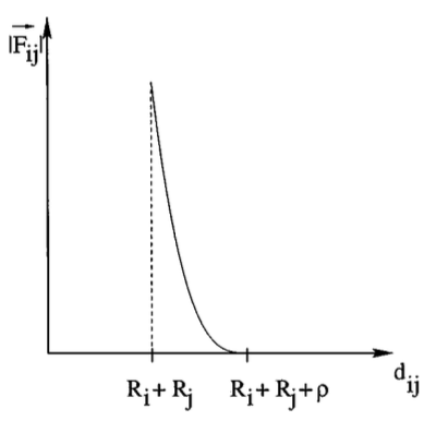
Figure 1. Repulsion force [Glowinski]

For \(d_{ij} = R_i + R_j\), one defines \(| \overrightarrow{ F_{ij} } | = \frac{c_{ij}}{\epsilon}\), where \(c_{ij}\) is a scaling factor and \(\epsilon > 0\) the collision parameter. We usually set \(\epsilon \approx h^2\), where \(h\) the mesh step.

One approach to define this type of repulsive force is given by :

\[\overrightarrow{ F_{ij} } = \frac{c_{ij}}{\epsilon} \left( \left( \frac{d_{ij}-R_i-R_j-\rho}{\rho} \right)^{-} \right)^2 \frac{\overrightarrow{ G_{i }G_j }}{d_{ij}} \mbox{,}\]

where \(a^{-} = \max\{0,-a\}\). The second term represents a quadratic activation term. The term \(\frac{\overrightarrow{ G_{i }G_j }}{d_{ij}}\) is the normalized vector between the centers of mass of two bodies and \(c_{ij}\) has the dimension of a force.

The authors of the articles [AIP_Advances], [Computers_Fluids] and [Wan_Turek] presented a model which prevents the spherical rigid bodies from getting too close, but which can also handle the overlapping of the latter. When one considers the same two spherical rigid bodies \(B_i\) and \(B_j\) of radius \(R_i\), \(R_j\) and center of mass \(G_i\), \(G_j\), then this model is given by:

\[F_{ij} = \begin{equation*} \left\{\begin{array}{rcl} 0 \;, \quad &\mbox{for }& d_{ij} > R_i + R_j + \rho , \\ \frac{1}{\epsilon}(G_i - G_j)(R_i + R_j + \rho - d_{ij})^2 \;, \quad &\mbox{for }& R_i+R_j \leq d_{ij} \leq R_i + R_j + \rho , \\ \frac{1}{\epsilon^{'}}(G_i - G_j)(R_i + R_j - d_{ij}) \;, \quad &\mbox{for }& d_{ij} < R_i + R_j . \end{array}\right.\;. \end{equation*}\]

where \(d_{ij}\) is the distance between the mass centers. The range of the repulsion force is usually equal to \(\rho = 0.5 \sim 2.5 h\), where \(h\) the mesh size. The two terms \(\epsilon\) and \(\epsilon^{'}\) are small stiffness parameters for these collisions. When the following three properties are verified:

\(\rho \approx h\), where \(h\) the mesh size.
\(\frac{\rho_b}{\rho_f}\) is of order 1, where \(\rho_p\) the density of the body and \(\rho_f\) the fluid density.
The fluid is sufficiently viscous.

then one can set \(\epsilon \approx h^2\) and \(\epsilon^{'} \approx h\).

This same model can be used to describe collisions between bodies and the domain boundaries:

\[F^{W}_{i} = \begin{equation*} \left\{\begin{array}{rcl} 0 \;, \quad &\mbox{for }& d_{i} > 2R_i + \rho , \\ \frac{1}{\epsilon_W}(G_i - G^{'}_i)(2R_i + \rho - d_{i})^2 \;, \quad &\mbox{for }& 2R_i \leq d_{i} \leq 2R_i + \rho , \\ \frac{1}{\epsilon^{'}_W}(G_i - G^{'}_i)(2R_i - d_{i}) \;, \quad &\mbox{for }& d_{i} < 2R_i . \end{array}\right.\;. \end{equation*}\]

\(G^{'}_i\) is the center of the nearest imaginary body on the other side of the boundary and \(d_i\) represents the distance between this center and the center of mass of the real rigid body. This is shown in the following figure:

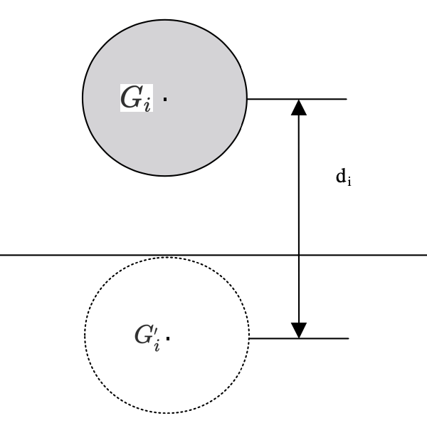
Figure 2. Spherical body - boundary collision [Multiphase_Flow]

The stiffness parameters \(\epsilon_W\) and \(\epsilon^{'}_W\) can be taken as \(\epsilon_W = \frac{\epsilon}{2}\) and \(\epsilon^{'}_W = \frac{\epsilon^{'}}{2}\).

The total repulsion force applied on the body \(B_i\) is then expressed by:

\[F_i = \sum_{j=1,j\neq i}^{N} F_{ij} + F_i^{W},\]

where \(N\) is the number of bodies. We will use this last model for our simulations.

2. Algorithm

In this part we will give the algorithm to compute the collision force applied to model the spherical body - spherical body and spherical body - boundary interactions. The parameters used in this model are specified in a json file and are thus available in the algorithm. Section Implementation contains more information about the parameters' definition and implementation. In our algorithm, the direct contact of the bodies is not considered, therefore we do not add the situation \(d_i < 2R_i\).

2.1. Specific algorithm with definition of bodies' and domain dimensions

First, we consider a specific algorithm: we define the radius of the body as well as the dimensions of the domain' box. We denote by \(N\) the number of rigid bodies, \(M = 4\) the number of walls and for simplicity we consider only bodies of same radius. The following algorithm is applied at each time step of the simulation.

\begin{algorithm}
    \caption{Specific algorithm for interactions between spherical bodies}
    \begin{algorithmic}
    \FUNCTION{contactforce}{}

    \STATE \Comment{Read the configuration file to define:}

    \STATE $\rho$ : collision force activation threshold.
    \STATE $\epsilon, \epsilon_W$ :  stiffness parameters.
    \STATE $r$ : radius of spherical rigid bodies.
    \STATE $h, w$ : height and width of the fluid domain.

    \STATE \Comment{Store the mass centers of the bodies:}

    \FOR{$1 \leq i \leq N$}
      \STATE $\mbox{massCenters}_{i} \leftarrow i$.massCenter()
    \ENDFOR

    \FOR{$1 \leq i \leq N$}

      \STATE \Comment{Stock the mass centers of imaginary bodies:}
      \STATE $\mbox{imaginary}_1 \leftarrow \{\mbox{massCenters}_{i}.x, h + r, \mbox{massCenters}_{i}.z \}$
      \STATE $\mbox{imaginary}_2 \leftarrow \{\mbox{massCenters}_{i}.x, - r, \mbox{massCenters}_{i}.z \}$
      \STATE $\mbox{imaginary}_3 \leftarrow \{-r, \mbox{massCenters}_{i}.y, \mbox{massCenters}_{i}.z \}$
      \STATE $\mbox{imaginary}_4 \leftarrow \{w + r, \mbox{massCenters}_{i}.y, \mbox{massCenters}_{i}.z \}$

      \FOR{$1 \leq j \leq M$}

        \STATE \Comment{Compute body-wall repulsion force:}

        \STATE $\mbox{dist}_{ij} \leftarrow ||\mbox{massCenters}_{i} - \mbox{imaginary}_j ||_2$
        \STATE $\mbox{activation} \leftarrow -(\mbox{dist}_{ij} - 2r - \rho)$

        \IF{activation $> 0$ \textbf{AND} $\mbox{dist}_{ij} > 2r$}
            \STATE $G_{ji} \leftarrow \mbox{massCenters}_{i} - \mbox{imaginary}_j$
            \STATE $F_{i}^W \leftarrow \frac{1}{\epsilon_W} (\mbox{activation})^2 G_{ji}$
            \STATE $F_i \leftarrow F_i + F_{i}^W$
        \ENDIF
      \ENDFOR

      \FOR{$i+1 \leq j \leq N$}
        \STATE \Comment{Compute body-body repulsion force:}
        \STATE $\mbox{dist}_{ij} \leftarrow ||\mbox{massCenters}_{i} - \mbox{massCenters}_{j} ||_2$
        \STATE $\mbox{activation} \leftarrow -(\mbox{dist}_{ij} - 2r - \rho)$

        \IF{activation $> 0$ \textbf{AND} $\mbox{dist}_{ij} > 2r$}
            \STATE $G_{ji} \leftarrow \mbox{massCenters}_{i} - \mbox{massCenters}_{j}$
            \STATE $F_{ij} \leftarrow \frac{1}{\epsilon} (\mbox{activation})^2 G_{ji}$
            \STATE $F_i \leftarrow F_i + F_{ij}$
        \ENDIF
      \ENDFOR
    \ENDFOR
    \RETURN  $F_i$
    \ENDFUNCTION
    \end{algorithmic}
\end{algorithm}

The vector \(F_i\) contains the repulsion force for each rigid body which is added to the right-hand side of Newton’s equation, describing the bodies' translation velocity.

2.2. Generalized algorithm

Secondly, we consider an algorithm that is still just applicable in the case of spherical bodies, but that is more generic than the first one. Instead of giving the radius of the spheres we compute the measure of the boundary of each body.

We then have:

\[\begin{align*} r &= \frac{\int_{\Gamma_b} 1}{2 \pi} \quad &\mbox{in dimension } 2 \mbox{ ,}\\ r &= \sqrt{\frac{\int_{\Gamma_b} 1}{4 \pi}} \quad &\mbox{in dimension } 3 \mbox{ ,} \end{align*}\]

where \(\Gamma_b\) the body boundary. The dimension and shape of the fluid domain are also no longer provided but the fast marching method is applied to obtain the distance between a body and the boundary of the domain. Information on this method is in section Repulsive force for arbitrary rigid bodies.

3. Test cases

There are different test cases for this type of collisions: the simulation of the contact between a spherical rigid body and the wall, between two spherical rigid bodies or between several rigid bodies in \(2\)D and \(3\)D. We will visualize our results from different test cases, obtained with the toolbox fluid of Feel++. For some simulations we compare them with the literature.

3.1. Validation : spherical rigid body - bottom collision in \(2\)D

We consider the sedimentation of a spherical rigid body in a vertical channel filled with an incompressible Newtonian fluid. The body falls under the effect of gravity towards the bottom of the channel. At initial time the fluid and the body are both at rest. The different parameters are defined as:

Name

Description

Values

\(\Omega\)

Computational domain (box)

[\(0,2\)] \(\times\) [\(0,6\)]

\(G\)

Body center

(\(1,4\))

\(\rho_d\)

Body density

\(1.25\)

\(r\)

Body radius

\(0.125\)

\(\rho_f\)

Fluid density

\(1\)

\(\mu\)

Fluid viscosity

\(0.1\)

\(\rho\)

Safety zone thickness

\(0.02\)

\(\epsilon_W\)

Stiffness parameter

\(0.0004\)

\(g\)

Gravity acceleration vector

\(\{ 0, -981 \}\)

\(\Delta t\)

Simulation time step

\(10^{-3}\)

\(h\)

Simulation mesh size

\(0.02\)

The graphs show the evolution in time of the vertical position of the body and of its vertical velocity obtained during the present work and in the article [Wan_Turek].

One can see that our results are close to the theoretical results. The difference in vertical velocity can be explained by a higher repulsive force intensity used for the literature results.

3.2. Application : spherical rigid body - wall collision in \(2\)D

Next, we consider the same test case by changing the direction of the gravity acceleration vector. We impose a rotation of angle \(\theta\) to the vector. The parameters that have been modified compared to the previous test case are given by:

Name

Description

Values

\(\epsilon_W\)

Stiffness parameter

\(0.00005\)

\(\theta\)

Rotation angle

\(-\frac{\pi}{4}\)

\(g\)

Gravity acceleration vector

\(\{981 \sin(\theta), -981 \cos(\theta) \}\)

\(\Delta t\)

Simulation time step

\(5*10^{-3}\)

\(h\)

Simulation mesh size

\(0.01\)

Under the effect of this gravity, the body will come into contact with the left wall. We will display its trajectory as well as the direction of the gravity vector at the times \(t = 0s\), \(t = 0.1s\), \(t=0.2s\) and \(t=0.3s\):

Figure 3. Body' trajectory

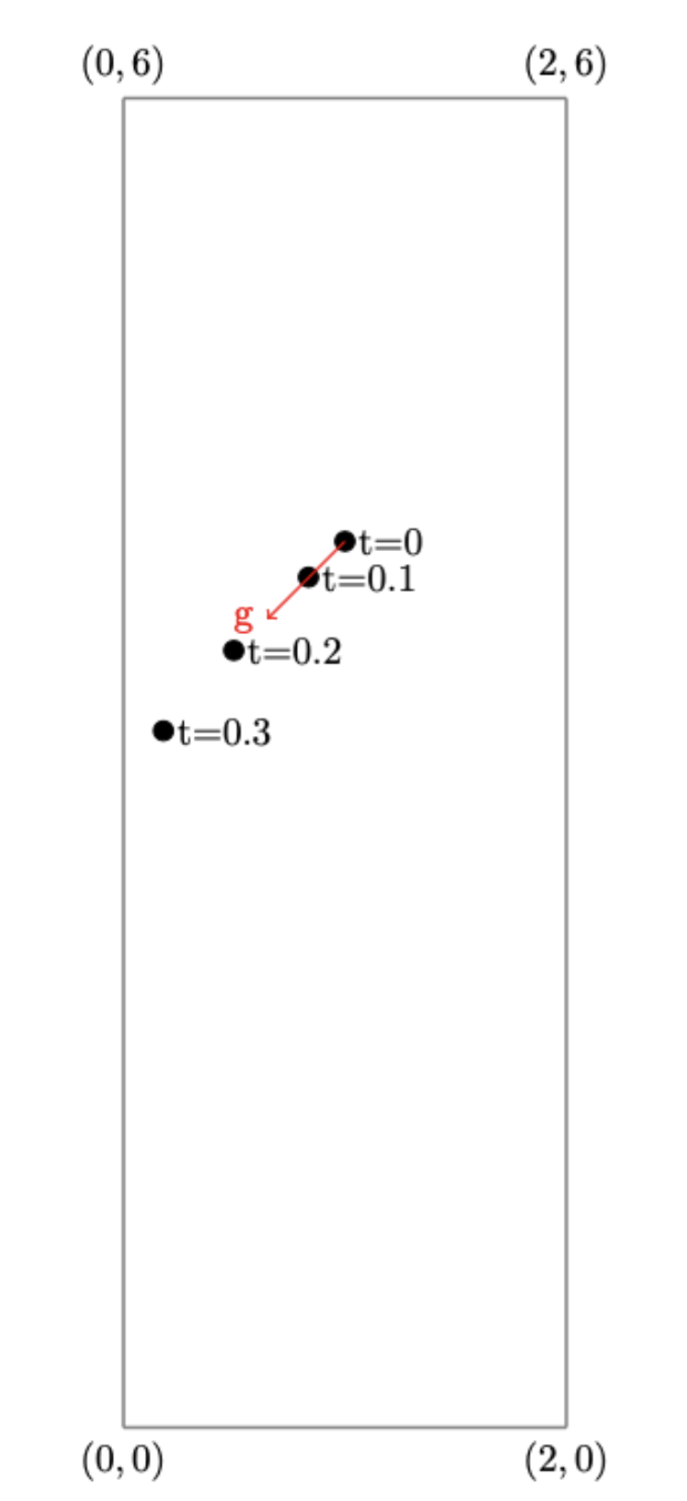
For this case, one expects that the horizontal position and the horizontal velocity of the body will be equal to zero after the contact point. By displaying these parameters over time one can observe these theoretical results.

3.3. Application : spherical rigid body - wall collision in circular box in \(2\)D

To show that our collision algorithm also works in the case of complex geometry, we consider the interaction between a spherical body and the wall of a circular box. The body is initially at rest and is located to the left of the domain center. It falls under the effect of gravity, and it is expected that at the end of the simulation the body is at the lowest point of the domain.

The four following figures show the trajectory of the body. It can be observed that the body continues to approach the lowest point of the domain after colliding with the boundary.

Figure 4. Body trajectory

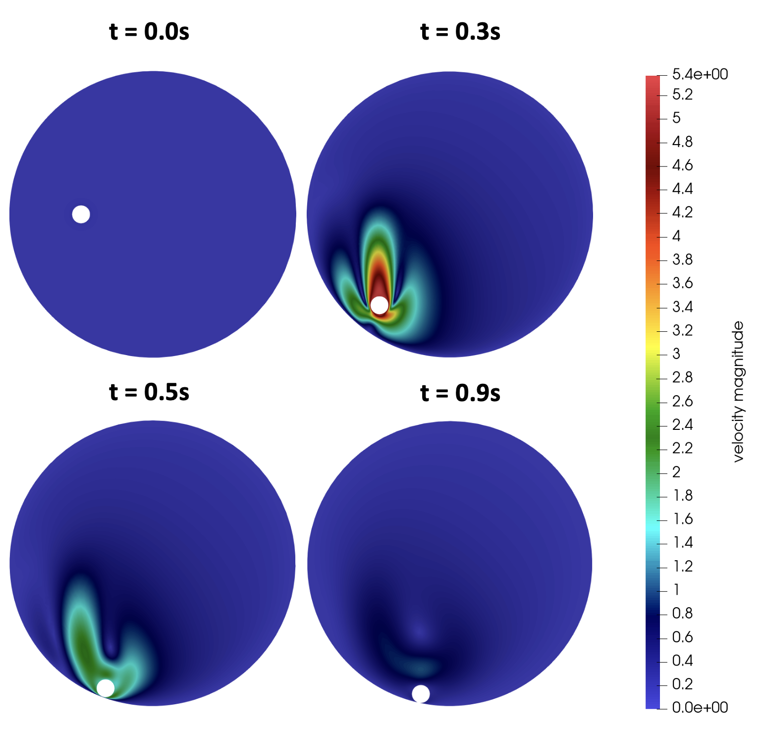
We can deduce that our implementation allows simulating body-boundary interactions in domains of arbitrary geometry.

3.4. Application : spherical rigid body - bottom collision in \(3\)D

In this test case we simulate the interaction between a sphere and the bottom of a box in three dimensions. The sphere is placed in an incompressible Newtonian fluid and falls under the effect of gravity. This simulation is presented in the article [Sphere_interaction] and the set of parameters is defined as:

Name

Description

Values

\(\Omega\)

Computational domain (box)

[\(0,4.919\)] \(\times\) [\(0,11.214\)] \(\times\) [\(0,14.919\)]

\(G\)

Body center

(\(2.457,10.1745,2.457\))

\(\rho_d\)

Body density

\(1.1.35\)

\(r\)

Body radius

\(0.315\)

\(\rho_f\)

Fluid density

\(1.195\)

\(\mu\)

Fluid viscosity

\(0.305\)

\(\rho\)

Safety zone thickness

\(0.25\)

\(\epsilon_W\)

Stiffness parameter

\(0.0005\)

\(g\)

Gravity acceleration vector

\(\{ 0, -981, 0 \}\)

\(\Delta t\)

Simulation time step

\(0.005\)

\(h\)

Simulation mesh size

\(0.125\)

The following two graphs, which represent respectively the vertical position and the vertical velocity of the sphere, show that this interaction is well simulated with our implementation. After the collision, the sphere remains close to the bottom and the velocity becomes zero. The results are close to the results of the literature. Thus, our model is also valid for three-dimensional simulations.

The sphere bounces slightly at the bottom of the box before reaching a stationary position. This can be observed by the vertical velocity of the body. The latter oscillates before becoming zero. The same behavior during a sphere-bottom interaction is present in the literature.

3.5. Application : spherical rigid body - spherical rigid body collision in \(2\)D

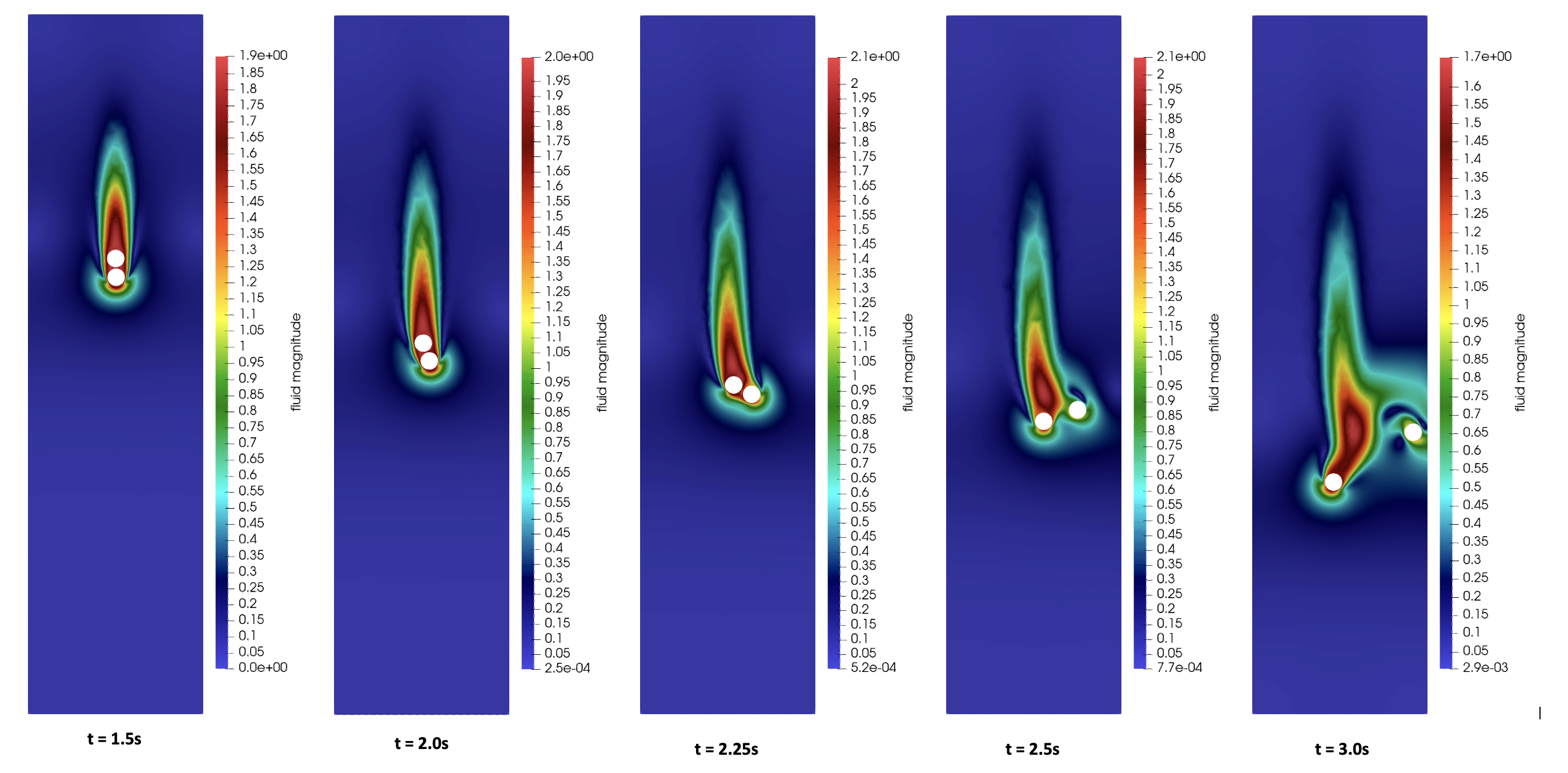
This well-known test case simulates the collision between two rigid bodies placed in a vertical channel filled with an incompressible Newtonian fluid. The bodies are initially at rest and then falling under the effect of gravity. The fluid velocity is \(0\) on the domain boundary. For this test case the behavior along a simulation of the bodies is given by the following figure:

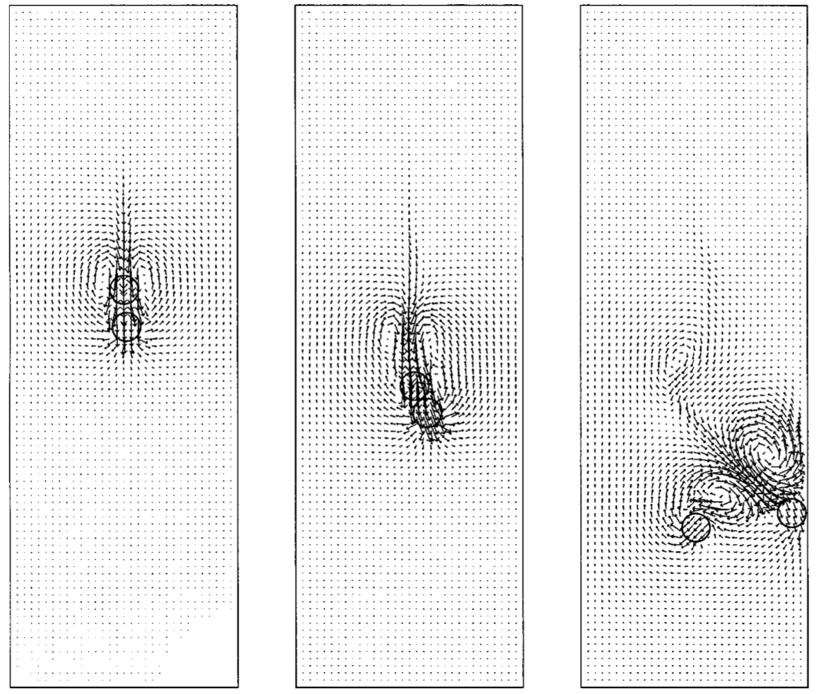
Figure 5. Displacement of the two bodies [Glowinski]

These simulations represent a phenomenon called drafting, kissing and tumbling : the lower body creates a pressure drop reducing the fluid resistance for the upper body. Therefore, the upper body falls faster until it collides with the lower one, leading to a rotation of the two latter. Finally, the repulsive forces cause the separation of the two bodies. We reproduce this phenomenon using the following parameters for the bodies and the fluid:

Name

Description

Values

\(\Omega\)

Computational domain

[\(0,2\)] \(\times\) [\(0,8\)]

\(O_L\)

Lower body center

(\(1,6.8\))

\(O_U\)

Upper body center

(\(0.999,7.2\))

\(d\)

Bodies diameter

\(0.2\)

\(\rho_s\)

Bodies density

\(1.01\)

\(\rho_f\)

Fluid density

\(1\)

\(\mu\)

Fluid viscosity

\(0.01\)

\(g\)

Gravity acceleration

\(\{ 0, -981 \}\)

The parameters of the repulsion force are fixed at :

Name

Description

Values

\(h\)

Mesh step

\(0.01\)

\(\Delta t\)

Time step

\(0.002\)

\(\epsilon\)

Stiffness parmeter for particle-particle collision

\(0.0001\)

\(\epsilon_W\)

Stiffness parmeter for particle-wall collision

\(0.00005\)

\(\rho\)

Safety zone thickness

\(0.025\)

We realize the simulation on the time interval [\(0s,5s\)]. By visualizing the position of the bodies at time instants \(t = 1.5s\), \(t = 2.0s\), \(t = 2.25s\), \(t = 2.5s\) and \(t = 3.0s\) one can observe the phenomenon drafting, kissing and tumbling :

Figure 6. Position of the two bodies

One can display the coordinates of the center of the two bodies over time:

This simulation has been frequently presented in the literature [Glowinski], [AIP_Advances], [Computers_Fluids], [Wan_Turek]. Results close to those of the literature are found, the differences come from the different definitions of collision forces.

3.6. Application : multi-collisions between spherical bodies in \(2\)D

As a last test case for spherical rigid bodies, we consider collisions between 100 bodies. This simulation is detailed in the article [Collision_simulations]. The fluid, bodies and collision parameters are listed in the following table:

Name

Description

Values

\(\Omega\)

Computational domain

[\(0,1\)]\(\times\)[\(0,2\)]

\(d\)

Bodies diameter

\(0.0625\)

\(\rho_d\)

Bodies density

\(1.01\)

\(\rho_f\)

Fluid density

\(1.0\)

\(\mu\)

Fluid viscosity

\(0.01\)

\(\rho\)

Safety zone thickness

\(0.025\)

\(\epsilon\)

Stiffness parmeter for particle-particle collision

\(0.000005\)

\(\epsilon_W\)

Stiffness parmeter for particle-wall collision

\(0.0000001\)

\(h\)

Mesh size

\(0.01\)

\(\Delta t\)

Time step

\(0.002\)

We illustrate the initial configuration as well as the evolution in time of the bodies positions by the following video:

One can observe that the bodies close to the right and left wall fall slower than the bodies initially located at the center. At final time, all bodies are settled at the bottom of the computational domain.

References on collision models

[Glowinski] R. Glowinski, T. W. Pan, T. I. Hesla, D. D. Joseph, and J. Périaux (2000). A Fictitious Domain Approach to the Direct Numerical Simulation of Incompressible Viscous Flow past Moving Rigid Bodies: Application to Particulate Flow. Download PDF
[AIP_Advances] K. Usman, K. Walayat, R. Mahmood, et al. (2018). Analysis of solid particles falling down and interacting in a channel with sedimentation using fictitious boundary method. Download PDF
[Computers_Fluids] L. Wang, Z.L. Guo, J.C. Mi (2014). Drafting, kissing and tumbling process of two particles with different sizes. Download PDF
[Wan_Turek] Decheng Wan and Stefan Turek (2004). Direct Numerical Simulation of Particulate Flow via Multigrid FEM Techniques and the Fictitious Boundary Method. Download PDF
[Multiphase_Flow] P. Singh, T.I Hesla, D.D Joseph (2002). Distributed Lagrange multiplier method for particulate flows with collisions.
[Settling_ellipsoid] Tsorng-Whay Pan, Roland Glowinski, Giovanni P.Galdi (2001). Direct simulation of the motion of a settling ellipsoid in Newtonian fluid. Download PDF
[FMM_1] J.A. Sethian (1996). A fast marching level set method for monotonically advancing fronts.
[FMM_2] J.A. Sethian (1996). Level Set Methods and Fast Marching Methods; Evolving Interfaces in Computational Geometry, Fluid Mechanics, Computer Vision and Materials Sciene.
[FMM_3] J.A. Sethian. Level Set Methods and Fast Marching Methods.
[CollisionModel_DNS] Ramandeep Jain, Silvio Tschisgale, Jochen Fröhlich (2019). A collision model for DNS with ellipsoidal particles in viscous fluid.
[DNS_Framework] S.Tschisgale, T.Kempe and J.Fröhlich (2018). A general implicit direct forcing immersed boundary method for rigid particles.
[Wu_Shu] J.Wu, C.Shu (2009). Particulate Flow Simulation via a Boundary Condition-Enforced Immersed Boundary-Lattice Boltzmann Scheme.
[Stenotic_artery] H.Li, H.Fang, Z.Lin, S.Xu, S.Chen (2004). Lattice Boltzmann simulation on particle suspensions in a two-dimensional symmetric stenotic artery.
[Collision_simulations] L.H. Juarez, R. Glowinski, T.W. Pan (2004). Numerical Simulation of Fluid Flow with Moving and Free Boundaries. Download PDF
[Collision_ellipticalParticle] Zhenhua Xia, Kevin W. Connington, Saikiran Rapaka, Pengtao Yue, James J. Feng, Shiyi Chen (2008). Flow patterns in the sedimentation of an elliptical particle. Download PDF
[Sphere_interaction] S.M. Dash, T.S. Lee (2015). Two spheres sedimentation dynmics in a viscous liquid column.
[MMG] www.mmgtools.org/mmg-remesher-try-mmg/mmg-remesher-tutorials/mmg-remesher-mmg2d/implicit-domain-meshing.