 .pdf
.pdf
The influence of the boundary on swimmers
1. Swimmer parallel to the wall
1.1. Introduction
In this example, we will investigate the influence of boundaries on swimmers. We will performe 10 simulation such that for each simulation, the center sphere of the swimmer is located at \((0,y)\), for \(i=0,2,..., 18\). As \(y\) increases, the swimmer gets closer from the wall. The idea behind performing all these simulations is to see the influence of the boundary on the dynamics of the swimmer and to show that the this influencthe the swimmer close enough to the boundary and see if its motion will be traped by walls depends on the distance between the swimmer and the wall.
1.2. geometry
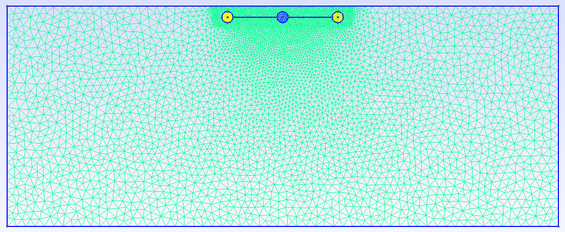
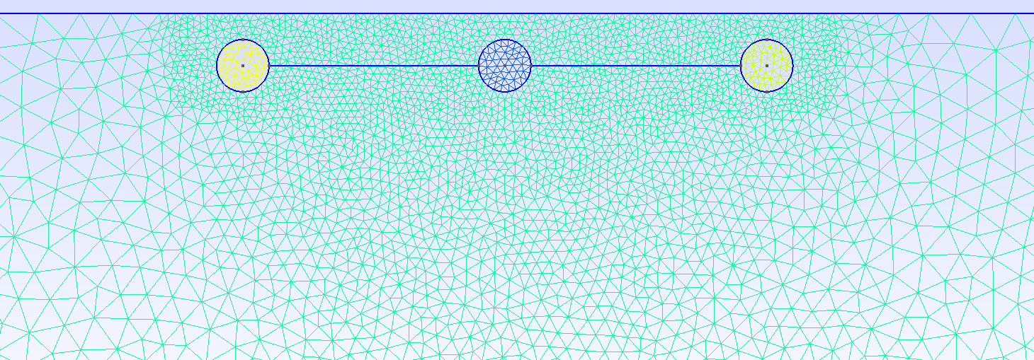
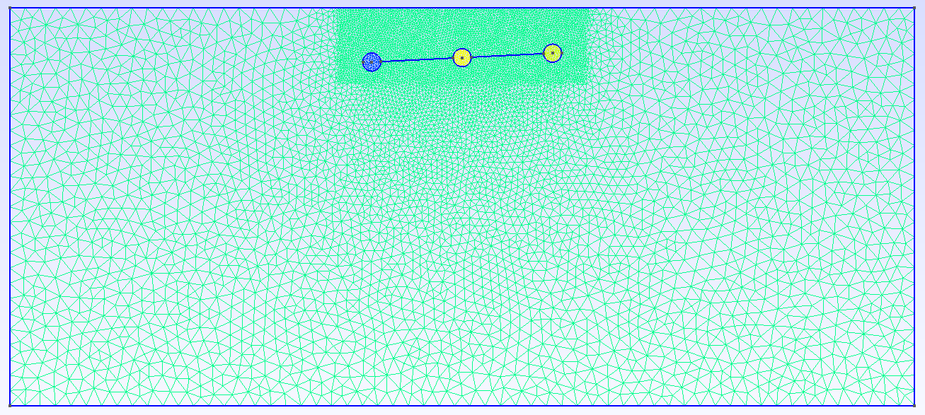
The domain geometry for \(y=18\) is shown in the figures below. The mesh is locally refined arround the swimmer.
1.4. Numerical results
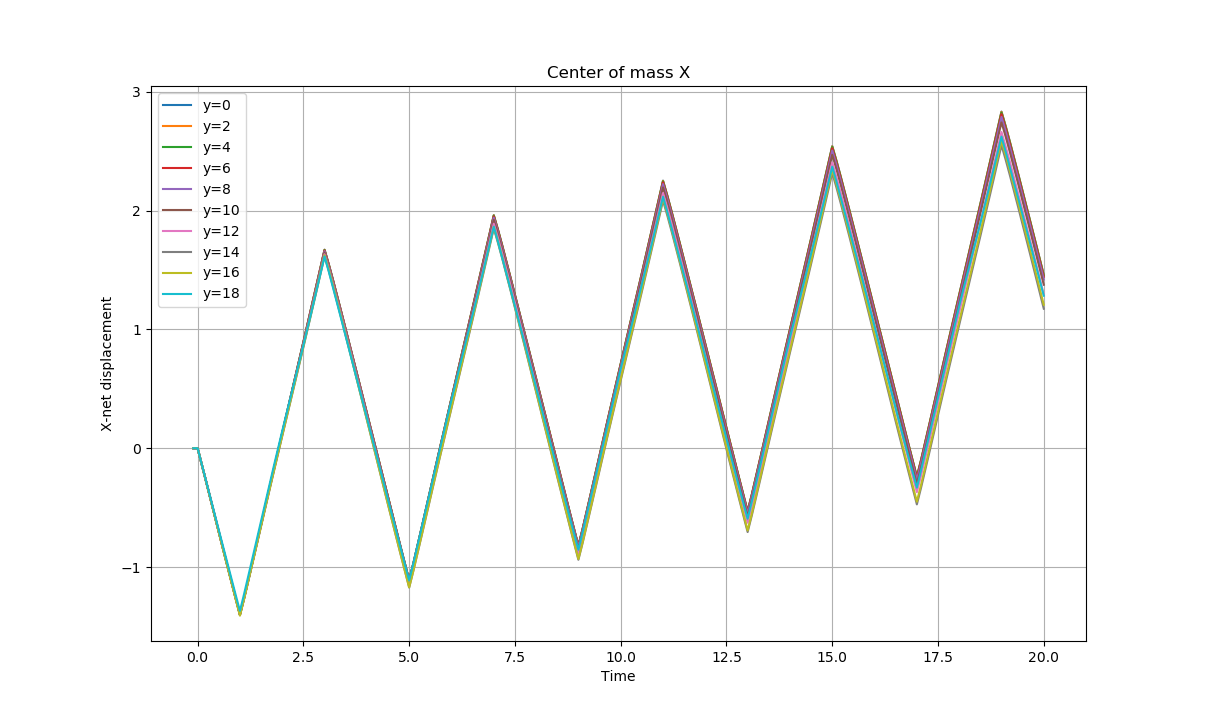
The results obtained by running the ten simulations are given in these figures :
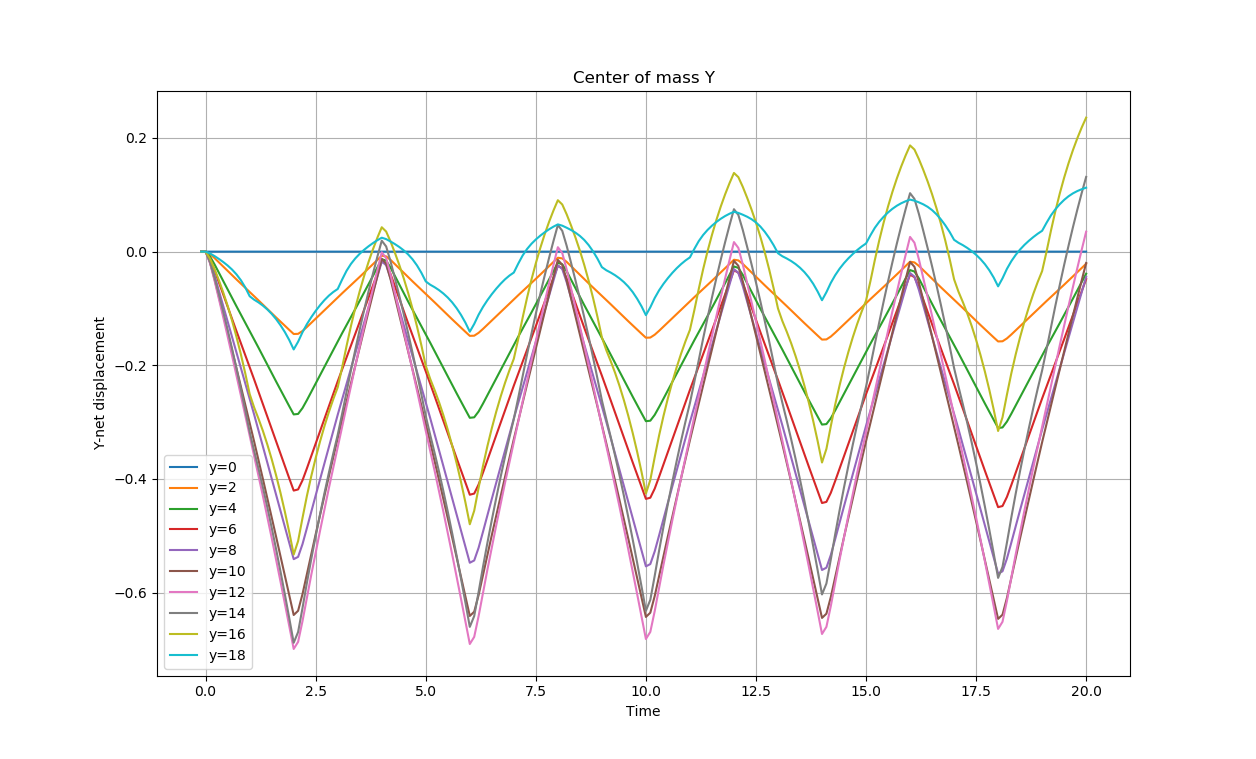
In the two following figures, we show, respectively, the swimmer’s net displacement with respect to \(X\) and \(Y\) of all \(y\)-positions in function of the time.
-
As a remark, we see that for \(y\leq 10\), the swimmer is pushed from the wall, while it is pulled to the wall for \(y>10\).
The two figures below show the net displacement gained at \(T_{final}=20 s\) in function of the swimmer’s position \(y\).
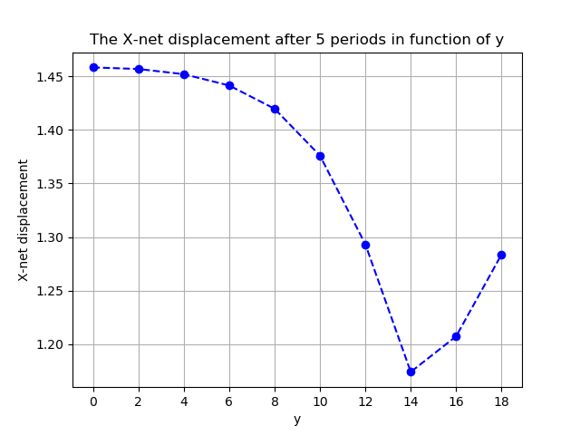
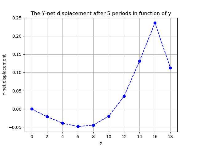
-
Here, we can see that the swimmer’s net displacement has a parabolic effect with respect to the distance from the wall. But for \(y>14\), the effect is not parabolic anymore and the behaviour of the swimmer changes.
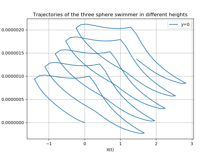
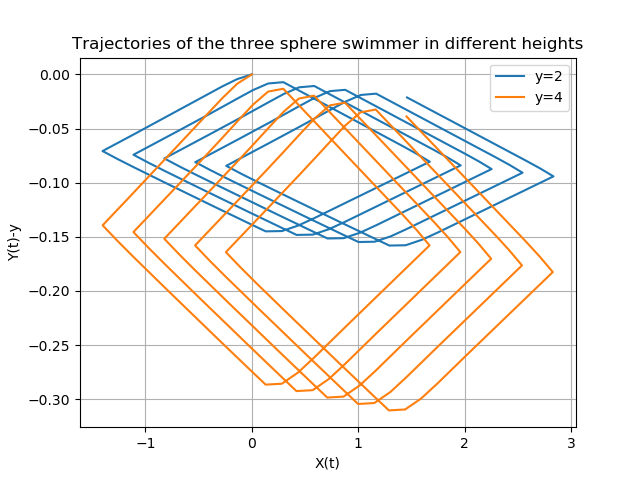
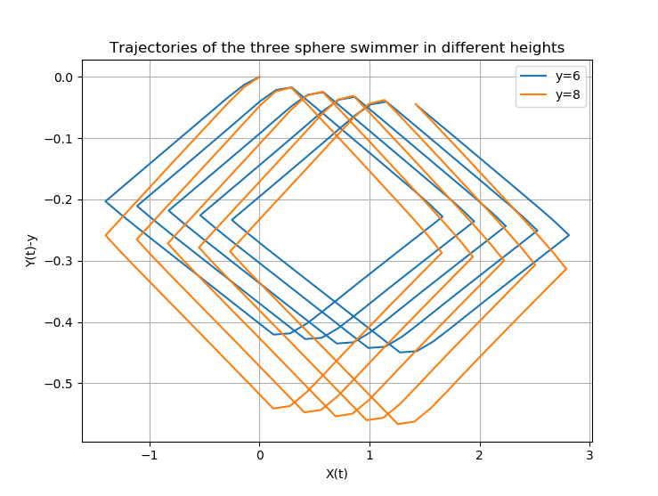
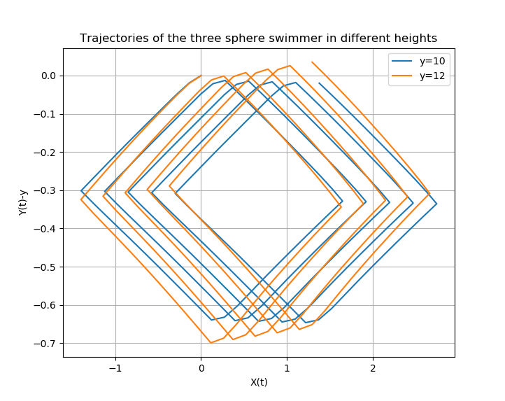
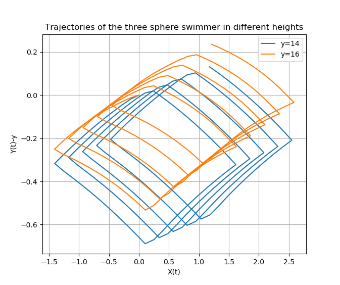
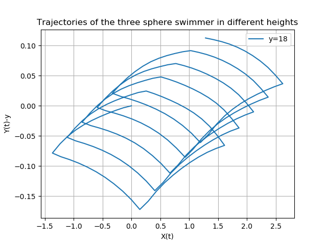
Here, we show the trajectories of the swimmer for each value of \(y\)
1.5. Stationary point
From the results above, we can see a trivial fixed point (with respect to \(Y\)-net dispacement) at \(y=0\). There is also another non trivial fixed point at the interval \([10, 12]\).
In the paper of Daddi-Moussa-Ider [Daddi-Moussa-Ider_2018], This non trivial fixed point is located at 0.8 of the channel’s width.
To determine this fixed point for our model, we generate 20 new simulations for \(y = 10, 10.1, 10,2,\cdots ,11.9, 12\).
The figure below shows the \(Y\)-net displacement for all \(y\) values mentioned above.
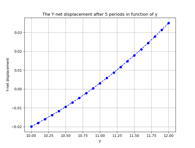
-
The non trivial fixed point is located at \(y\approx 10.9\), which is 0.78 of the channel’s width.
Note that by the symmetry of the channel domain, another fixes point should be locatd at \(y=-10.9\) (0.22 of the channel’s width).
2. Swimmer with an angle \(\theta\) with the horizon
2.1. Introduction
In this section, we study the influence of the wall on a 3D three sphere swimmer whose arm makes an angle \(\theta\) with the horizon as illustrated below :
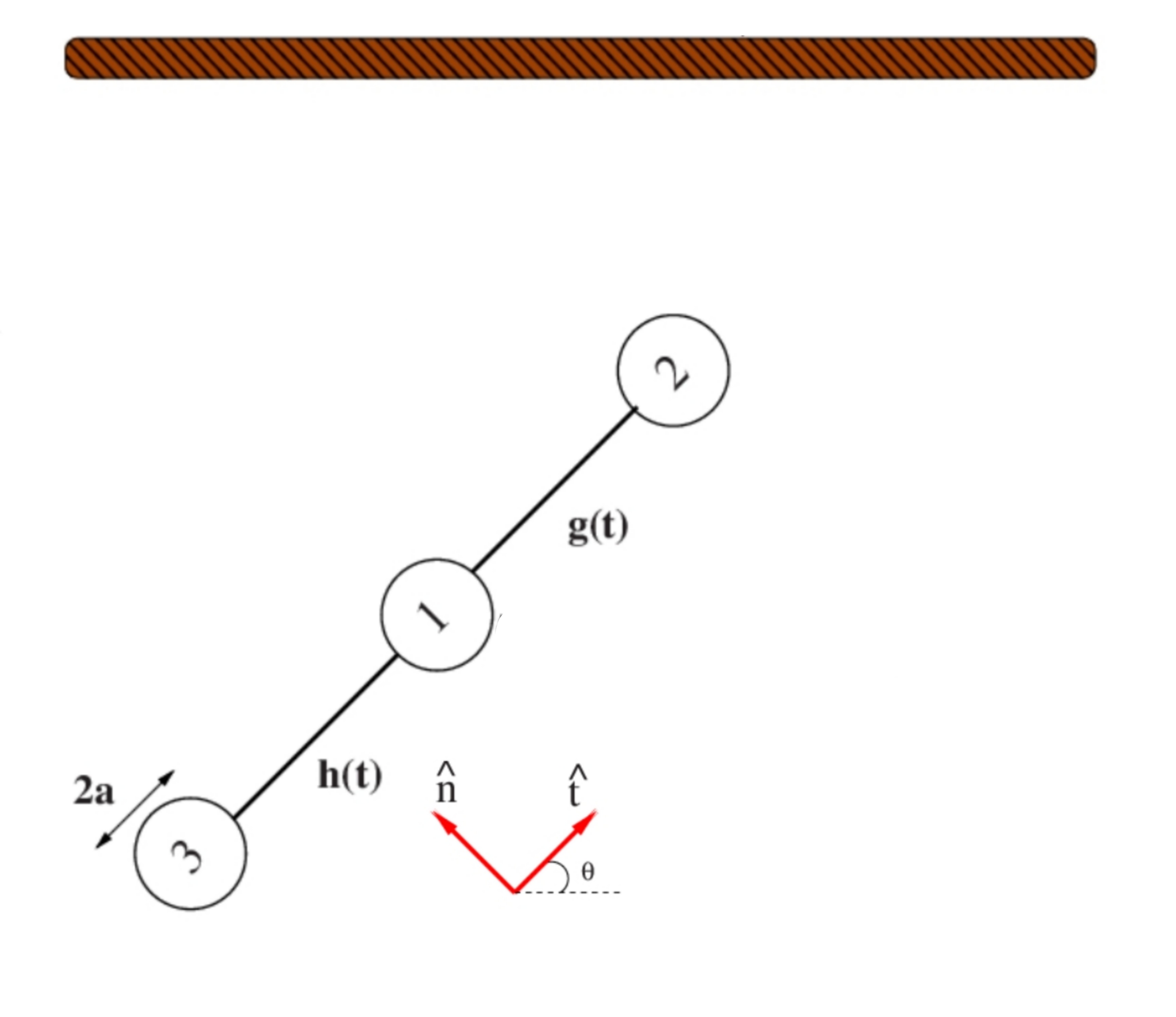
where \(g(t)= L+u_1(t)\) and \(h(t)= L+u_2(t)\).
2.2. Literature review
This model has been studied by Zargar and Najafi in their paper [Zargar_2009] and theoritical results were proposed. The functions \(u_1\) and \(u_2\) in Najafi’s paper are taking the fom :
\[ \begin{cases} u_1(t)=u_{10}cos(\omega t)\\ u_2(t)=u_{20}cos(\omega t + \phi) \end{cases} \]
and the swimmer velocity and the angle \(\theta\) are given as follow :
\[ \begin{cases}\displaystyle{ v_x = -\frac{1}{16} \left(\frac{R}{L^{2}} \right)\left[\theta ^{2} + 93 \left(\frac{y}{L}\right) ^2 \right] \mathbf{\Phi},\\ v_y = \frac{3}{16} \left(\frac{R}{L^{2}} \right)\left[ \theta ^{3} - \theta \left(\frac{y}{L}\right) ^2 \right] \mathbf{\Phi},\\ \dot{\theta} = \frac{105}{16}\left(\frac{R}{L^3} \right) \theta ^2 \left(\frac{y}{L} \right) \mathbf{\Phi},} \end{cases} \]
where \(\mathbf{\Phi} = <u_1 \dot{u_2}-u_2 \dot{u}_1>\) denotes the averaging over a complete cycle of deformations.
In our example, the path deformation is not the same as the one proposed in Zagar’s paper. The path deformation we consider in this example is given as follow :
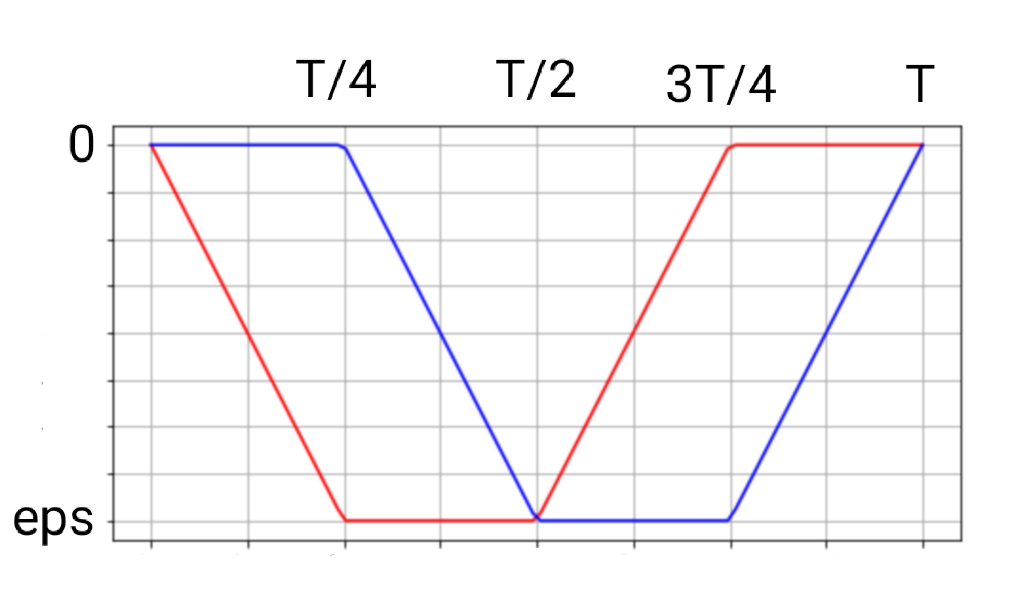
The analytical forms of \(u_1\) and \(u_2\) over one period is given as follow :
\[ u_1(t) =\begin{cases} -\frac{4}{T}\varepsilon t\qquad\qquad \text{if } t\in[0,\frac{T}{4}],\\ -\varepsilon \qquad\qquad\;\;\;\; \text{if } t\in[\frac{T}{4},\frac{T}{2}],\\ \frac{4}{T}\varepsilon t - 3\varepsilon\qquad\;\; \text{if } t\in[\frac{T}{2},\frac{3T}{4}],\\ 0\qquad \qquad\qquad\text{if } t\in[\frac{3T}{4},T] \end{cases} \]
and
\[ u_2(t) =\begin{cases} 0\qquad\qquad\qquad \text{if } t\in[0,\frac{T}{4}],\\ -\frac{4}{T}\varepsilon t + \varepsilon\qquad\; \text{if } t\in[\frac{T}{4},\frac{T}{2}],\\ -\varepsilon \qquad\qquad\;\;\;\; \text{if } t\in[\frac{T}{2},\frac{3T}{4}],\\ \frac{4}{T}\varepsilon t - 4\varepsilon\qquad\;\; \text{if } t\in[\frac{3T}{4},T]. \end{cases} \]
Then,
\[\mathbf{\Phi} = <u_1 \dot{u_2}-u_2 \dot{u}_1> = \frac{8\varepsilon^2}{T}.\]
Hence, the velocity filed and the angle \(\theta\) takes the previous form with :
\[\mathbf{\Phi} = \frac{8\varepsilon^2}{T}.\]
Here are some important points in the Zargar’s paper [zargar_2009] :
-
The velocities \(v_x\) and \(v_y\) are proportional to \(\frac{1}{L^2}\) When the swimmer is far from the wall.
-
The velocities \(v_x\) and \(v_y\) are proportional to \(\frac{1}{L^4}\) When the swimmer is close to the wall.
-
The swimmer orients itself parallel to the wall wherever the swimmer exists (close to or far from the wall).
2.3. Geometry
Here, we create a three sphere swimmer with an angle \(\theta\) in a rectangular channel of dimensions \([-L,L]\times [-l,l]\). The geometry is illustrated below.
2.4. Input parameters
Name |
Description |
values |
Unit |
\(\theta\) |
angle with the horizon |
\(\displaystyle{\frac{\pi}{64}}\) |
\(radian\) |
\((x_c, y_c)\) |
initial center of mass |
(0, 14.5) |
\(\mu m\) |
\([-L,L]\times [-l,l]\) |
rectangle dimension |
\([-50,50]\times[-20,20]\) |
\(\mu m\times\mu m\) |
2.5. Numerical reuslts
First, we want to check if the swimmer will orient itself parallel to the as the case for [Zargar_2009]. For this, we present here the numerical results obtained using the feelpp fluid toolbox.
The following figures show the center of mass and \(Y\)-displacement for the three spheres.
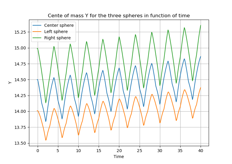
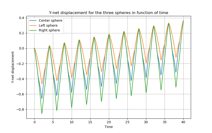
-
As a remark, we can see that unlike the parallel case of the swimmer, here the \(Y\)-net displacement amplitudes of the three spheres are not equal. This is not surprising since we have shown in the first section (swimmer parallel to the wall) that the amplitude of Y-displacement depends on the position of the swimmer. Here, the spheres are not at the same \(y\) position which makes the results seem to be convinient.
The \(Y\)-net displacement of each sphere in function of periods is shown in the figure below :
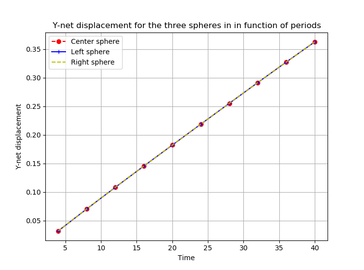
-
The last figure shows that the swimmer’s arms are still making the angle \(\theta\) with the horizon, while in the Literature, the swimmer oreints itself parallel to the wall.
References on Swimmers near a wall
-
[Daddi-Moussa-Ider_2018] Daddi-Moussa-Ider, Abdallah, Maciej Lisicki, Arnold J. T. M. Mathijssen, Christian Hoell, Segun Goh, Jerzy B\lawzdziewicz, Andreas M. Menzel, and Hartmut Löwen. State Diagram of a Three-Sphere Microswimmer in a Channel. Journal of Physics: Condensed Matter 30, no. 25 (June 2018): 254004. doi.org/10.1088/1361-648x/aac470. Download PDF
-
[Zargar_2009] R. Zargar,A. Najafi, M. Miri. Three-sphere low-Reynolds-number swimmer near a wall, Phys. Rev. E (2009). doi.org/10.1103/PhysRevE.80.026308 Download PDF