Repulsive force for arbitrary rigid bodies

Table of Contents

1. Tools : Fast Marching methods
2. Mathematical formulation
3. Algorithm
4. Test cases
References on collision models

1. Tools : Fast Marching methods

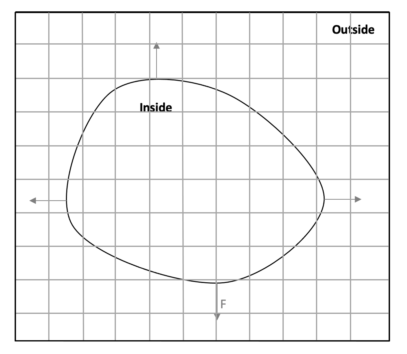
When considering complex shaped bodies, one can no longer compute the distance between the bodies using the coordinates of their center of mass. To fix this problem, the Fast Marching method is used to compute the distance field with respect to the boundary of a body.

The fast marching method is a level set algorithm introduced by J. A. Sethian [FMM_1],[FMM_2] and [FMM_3]. Level set methods are partial-differential-equations-based numerical techniques for tracking the evolution of interfaces: either a curve in two dimensions or a surface in three dimensions. The fast marching method is a specific approach of level set techniques. The front is propagating in a direction normal to itself with a speed everywhere positive or negative. This method is used in our collision algorithms to compute the distance between the boundaries of bodies or between the boundaries of a body and the fluid domain. We will explain the mathematical formulation and some test cases of this fast marching method.

1.1. Mathematical framework

Consider a curve separating one region (inside region) form another (outside region) and propagating with a positive speed $F$ normal to itself. The speed $F$ can depend on many factors, such as the geometric information, the shape and position of the front and on physical effects.

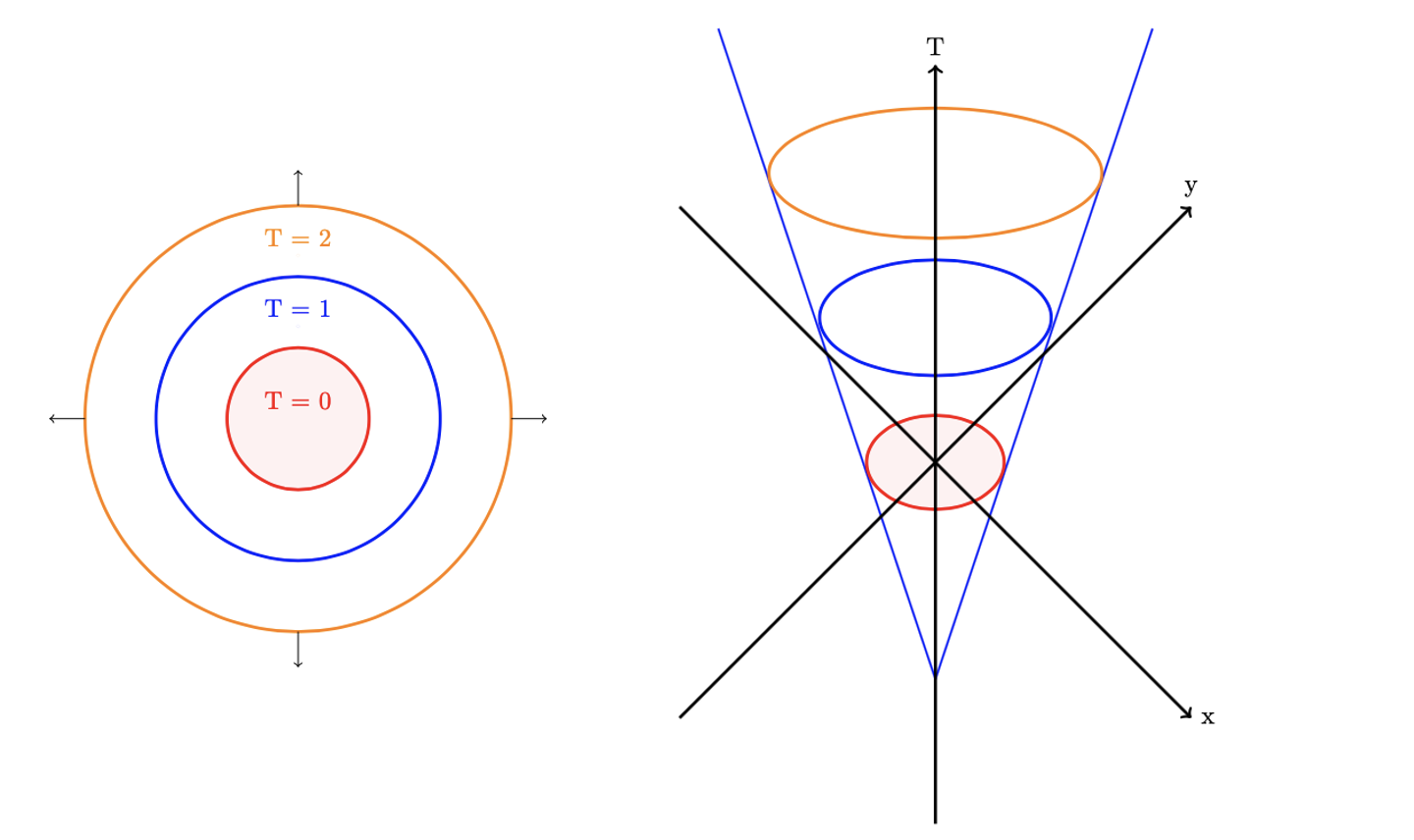
The fast marching method characterizes the evolution of the curve by computing the arrival time $T(X)$ of the interface crossing each point $X \in \mathbb{R}^d$ of the grid, where $d = 2$ or $d = 3$:

Figure 1. Grid for propagating curve

The approach converts the moving boundary problem to a stationary formulation. The coordinate system remains fixed and at each point $X \in \mathbb{R}^d$, where $d = 2$ or $d = 3$, the arrival time function:

\[\begin{array}{lrcl} T : & \mathbb{R}^d & \longrightarrow & \mathbb{R} \\ & X & \longmapsto & T(X) = t \end{array}\]

returns the time $t$ at which the interface crosses it. Hence, $T(X)$ is in one higher dimension than the original problem and gives a surface intersecting the plane where the curve is initially. At any height $t$, this surface gives the set of points reached at time $t$.

One can easily describe the problem in one dimension. The distance is expressed as the product of speed and time, therefore:

\[1 = F \frac{dT}{dx}\]

This aspect is applied in two and three dimensions: the gradient of arrival time surface is inversely proportional to the speed. Using a speed $F=1$ (respectively $F=-1$), the arrival time surface corresponds to the distance field of the outside region (respectively inside region).

Let $\Gamma$ be the initial location of the curve, called the zero level, propagating in a direction normal to itself with speed $F$, the fast marching method characterizes the front distance field as the solution to the following boundary value problem:

\begin{align*} | \nabla T| F &= 1, \\ T &= 0 \quad \mbox{on } \Gamma . \end{align*}

where $F = 1$ or $F = -1$.

As an example, one can consider a circular front propagating with constant speed $F=1$. The arrival time surface is given by the following cone-shaped figure:

Figure 2. Circular propagating front with speed $F=1$

The fast marching algorithm adds one dimension to the initial problem, hence it is computationally expensive. The narrow band approach provides an efficient modification by computing the arrival time $T(X)$ only in a near neighborhood of the zero level. This neighborhood is set by a predefined threshold. Once this threshold is crossed, the narrow band approach adopts an arbitrary value corresponding to the maximum value reached.

1.2. Test cases in $2$D

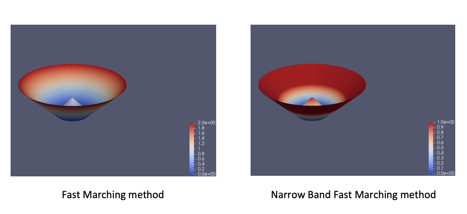
To test the implementation of the fast marching method and the narrow band approach, we consider the same circular front as before with a maximal arrival time $T=2$. Thus, we consider three circles of radius $r=1, r=2$ and $r=3$. We apply the fast marching method to the inner circle and the narrow band approach with a threshold corresponding to the boundary of the center circle. One can visualize the distance field, i.e. the arrival time surface, obtained with a constant speed $F=1$ for the outside region of the inner circle and $F=-1$ for the inside region of the inner circle:

For this configuration, we will first compare the error in $L_2$ norm for different mesh sizes, executing in sequential. We show in the table the mesh size, the number of mesh elements, the error obtained for the two approaches and the orders of convergence:

Mesh size

Mesh elements

Fast marching method - error

Order

Narrow band approach - error

Order

$0.4$

$472$

$0.228221$

$0.114242$

$0.2$

$1828$

$0.10512$

$1.12$

$0.0486447$

$1.23$

$0.1$

$6890$

$0.0460018$

$1.19$

$0.0205917$

$1.24$

$0.05$

$26712$

$0.0225448$

$1.02$

$0.00964262$

$1.09$

$0.025$

$105940$

$0.0107953$

$1.06$

$0.00467771$

$1.04$

$0.0125$

$420246$

$0.00509793$

$1.08$

$0.00229392$

$1.03$

$0.00625$

$1676726$

$0.00265853$

$0.94$

$0.00114032$

$1.00$

We obtain for both approaches an order of convergence equal to $1$, which corresponds to the theoretical value.

As a second test, we use the same geometry. We set the mesh size to $h = 0.01$ and we parameterize the bandwidth $\delta$. The goal is to observe an increasing execution time with an increasing band thickness.

The visualizations for different thresholds for the band thickness are given by:

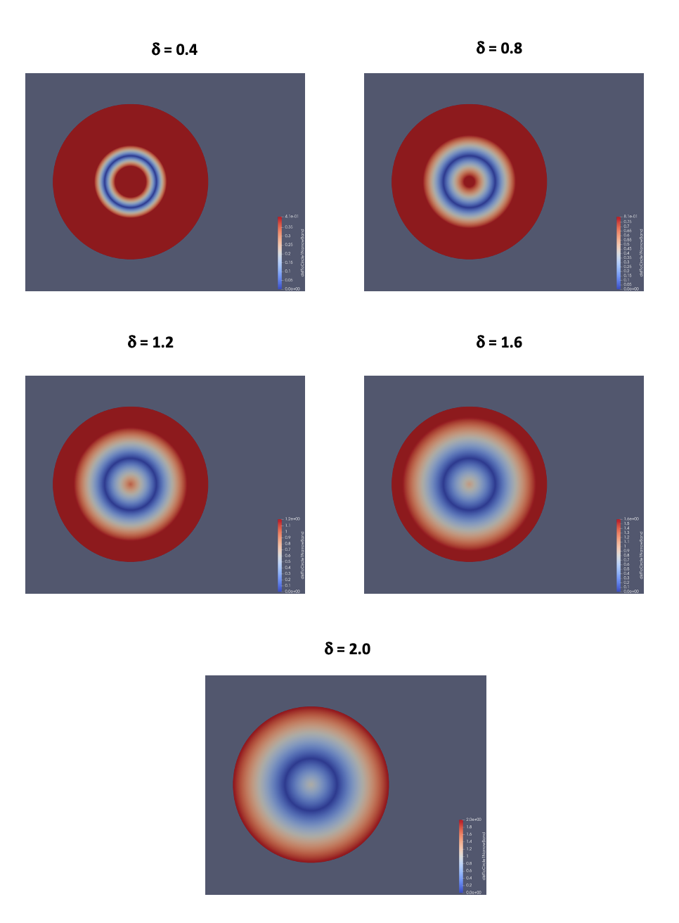
The following table contains the number of mesh elements, the number of mesh elements of the band, the execution time and the bandwidth:

Global mesh elements

Band mesh elements

Narrow band approach - execution time

Bandwidth

$656170$

$70576$

$0.781$s

$\delta=0.4$

$656302$

$163590$

$1.513$s

$\delta=0.8$

$655924$

$280212$

$2.492$s

$\delta=1.2$

$657032$

$419562$

$3.564$s

$\delta=1.6$

$668856$

$582398$

$5.315$s

$\delta=2.0$

We can observe that the execution time of the narrow band method increases with the width of the band. To better observe it we plot the execution time as a function of the bandwidth:

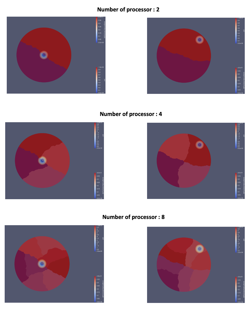
The last test case in $2$D analyzes the influence of partitioning on the execution time when running the fast marching method and narrow band approach in parallel. We consider two different geometries. The first one consists of three centered circles of radius $r=0.1$, $r=0.5$ and $r=3.0$. The second one contains the same three circles, but the center of the small circle and the middle circle is at coordinates $(1.75,1.75)$. We apply the narrow band approach to the boundary of the small circle and give as bandwidth the distance to the boundary of the middle circle, thus the threshold is $0.4$. The mesh size is set to $0.01$. The number of global mesh elements of the geometry with centered circles is $656084$ and the number of mesh elements of the band is $17898$. With non-centered circles the number of global mesh elements is $656776$ and of the band $17912$. The values of all these parameters are listed in the following table:

Name

Description

Values

$r_s$

Radius of small cercle

$0.1$

$r_m$

Radius of middle cercle

$0.5$

$r_l$

Radius of large cercle - domain

$3.0$

$O_c$

Center of centerd circles

$(0,0)$

$O_{nc}$

Center of non-centerd circles

$(1.75,1.75)$

$\delta$

Bandwidth

$0.4$

$h$

Mesh size

$0.01$

Global mesh elements centered circles

$656084$

Global mesh elements non-centered circles

$656776$

Band mesh elements centered circles

$17898$

Band mesh elements non-centered circles

$17912$

As the circles of the geometries have different center coordinates, the partitioning is different as well. We will visualize the partitioning of the two geometries for a number of processors equal to $2,4$ and $8$ and display the execution time.

The visualization of the partitioning for the centered circles (left) and the non-centered circles (right) are given by:

The following table shows the execution times:

Number of processor

FMM - Centered circles

Narrow band FMM - Centered circles

FMM - Non-centered circles

Narrow band FMM - Non-centered circles

$1$

$5.398$s

$0.102$s

$4.743$s

$0.090$s

$2$

$20.966$s

$0.123$s

$5.712$s

$0.101$s

$4$

$15.305$s

$0.109$s

$16.448$s

$0.135$s

$8$

$12.714$s

$0.108$s

$19.238$s

$0.090$s

One can notice that the parallel execution and thus the partitioning increases the execution time for the narrow band method. The execution times measured for the two geometries show that in general a partitioning that crosses the narrow band domain is more expensive than the case where this domain is computed by a single processor.

For the geometry of the centered circles we will analyze the influence of the domain size on the execution time of the narrow band approach. We keep the same radius for the small and the middle circle, $r=0.1$ and $r=0.5$, and we vary the radius of the large circle. The narrow band approach is still applied to the boundary of the small circle and the threshold is fixed by the boundary of the middle circle. The mesh size for these simulations is set to $0.01$ and the number of mesh elements of the band is $18214$.

Name

Description

Values

$r_s$

Radius of small cercle

$0.1$

$r_m$

Radius of middle cercle

$0.5$

$O_c$

Center of circles

$(0,0)$

$\delta$

Bandwidth

$0.4$

$h$

Mesh size

$0.01$

Band mesh elements

$18214$

We will show in the following table the total number of mesh elements, the radius of the large circle and the execution time of the narrow band approach for different numbers of processors:

Global mesh elements

Domain radius

Proc 1

Proc 2

Proc 4

Proc 8

$658350$

$r = 3$

$0.108$s

$0.126$s

$0.116$s

$0.114$s

$166282$

$r = 1.5$

$0.083$s

$0.112$s

$0.079$s

$74886$

$r = 1$

$0.072$s

$0.126$s

$0.089$s

$0.069$s

$42664$

$r = 0.75$

$0.067$s

$0.095$s

$0.078$s

$0.068$s

$22096$

$r = 0.5$

$0.069$s

$0.128$s

$0.099$s

$0.083$s

One can observe that the shortest execution times are obtained for a domain of radius $r=0.75$, which corresponds approximately to twice the threshold for the narrow band approach.

1.3. Test cases in $3$D

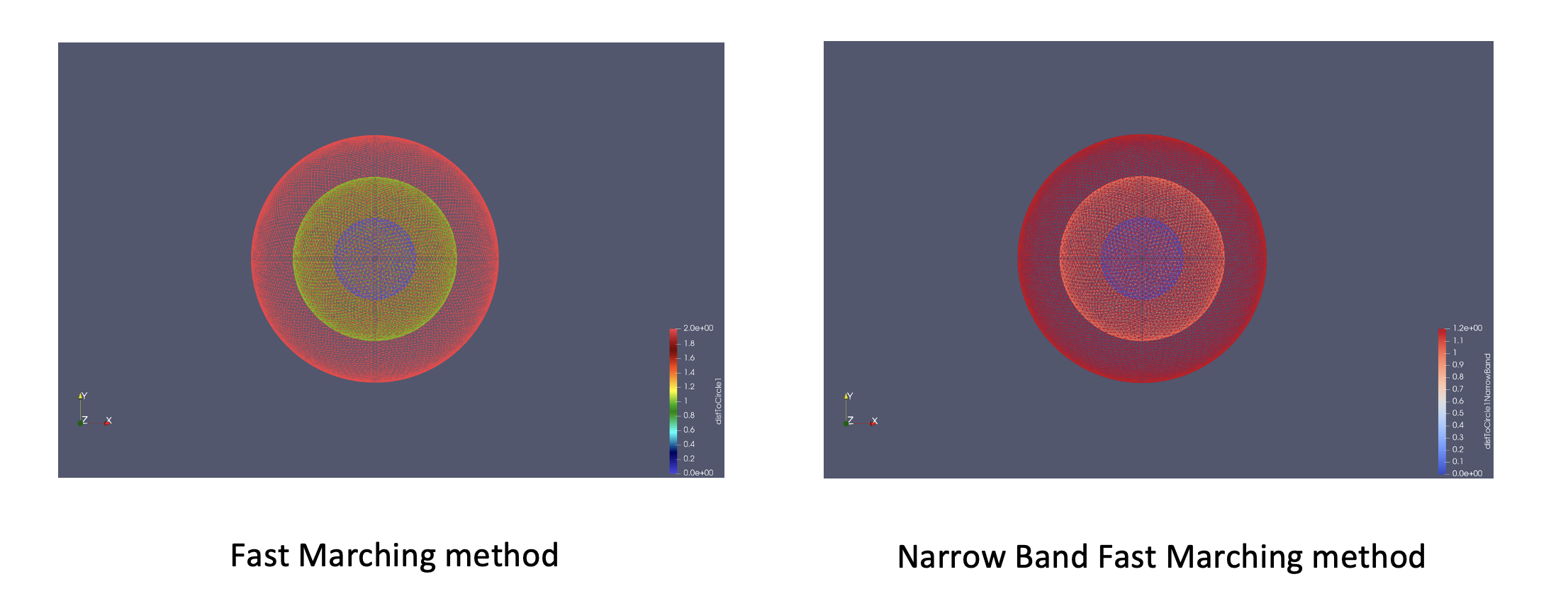
In the first three-dimensional test, we compare the error in $L_2$ norm and the execution time for different mesh sizes of the fast marching method and the narrow band approach. We consider three spheres of radius $r=1, r=2$ and $r=3$ and we apply the fast marching method to the inner sphere. The threshold of the narrow band approach corresponds to the boundary of the center sphere.

Using a mesh size equal to $h=0.1$, the representation of the distance function for both methods is given by the following figure:

We show in the table the mesh size, the number of global mesh elements and band mesh elements, the error obtained for the two approaches, the orders of convergence and the execution time. All simulations are performed in sequential.

Mesh size

Mesh elements

Band elements

FMM - time

FMM - error

FMM - Order

Nb - time

Nb - error

Nb - Order

$0.8$

$1489$

$434$

$0.011$s

$1.145115$

$0.003$s

$0.383392$

$0.4$

$8967$

$2606$

$0.069$s

$0.536080$

$1.09$

$0.018$s

$0.159507$

$1.27$

$0.2$

$69966$

$18942$

$0.719$s

$0.204597$

$1.39$

$0.109$s

$0.075742$

$1.07$

$0.1$

$540257$

$142808$

$9.186$s

$0.076191$

$1.42$

$1.810$s

$0.033052$

$1.20$

$0.05$

$4145185$

$1089447$

$76.254$s

$0.030112$

$1.34$

$17.854$s

$0.015853$

$1.06$

$0.025$

$32679043$

$8531962$

$1035.66$s

$0.012511$

$1.27$

$211.320$s

$0.007285$

$1.12$

The table proves that we find the appropriate orders of convergence. It can also be seen that the computational costs, increasing rapidly when the mesh size becomes small, are lower for the narrow band approach.

For the last test, we consider the same configuration used in the previous case. The inner and middle sphere have respectively a radius of $r = 0.1$ and $r = 0.5$. In order to analyze the influence of the width of the zone on which the default value of the narrow band approach is applied on the computation time, we vary the radius of the outer sphere. The mesh size is fixed to $h = 0.05$ and the number of mesh elements of the band is $23643$.

Name

Description

Values

$r_s$

Radius of small sphere

$0.1$

$r_m$

Radius of middle sphere

$0.5$

$O_c$

Center of circles

$(0,0)$

$\delta$

Bandwidth

$0.4$

$h$

Mesh size

$0.05$

Band mesh elements

$23643$

The following table gives the total number of mesh elements, the radius of the outer sphere (domain) and the execution time of the narrow band approach for different numbers of processors:

Total mesh elements

Domain radius

Proc 1

Proc 2

Proc 4

Proc 8

$4129925$

$r = 3$

$0.310$s

$0.768$s

$0.266$s

$0.182$s

$540854$

$r = 1.5$

$0.150$s

$0.525$s

$0.110$s

$0.082$s

$163522$

$r = 1$

$0.134$s

$0.426$s

$0.099$s

$0.058$s

$73274$

$r = 0.75$

$0.129$s

$0.362$s

$0.089$s

$0.062$s

It can be observed that the execution time decreases with decreasing radius of the outer sphere. One can conclude that the size of the domain has an influence on the execution time even by only modifying the width of the zone on which the default value of the narrow band approach is applied.

2. Mathematical formulation

Figure 3. Complex shaped bodies

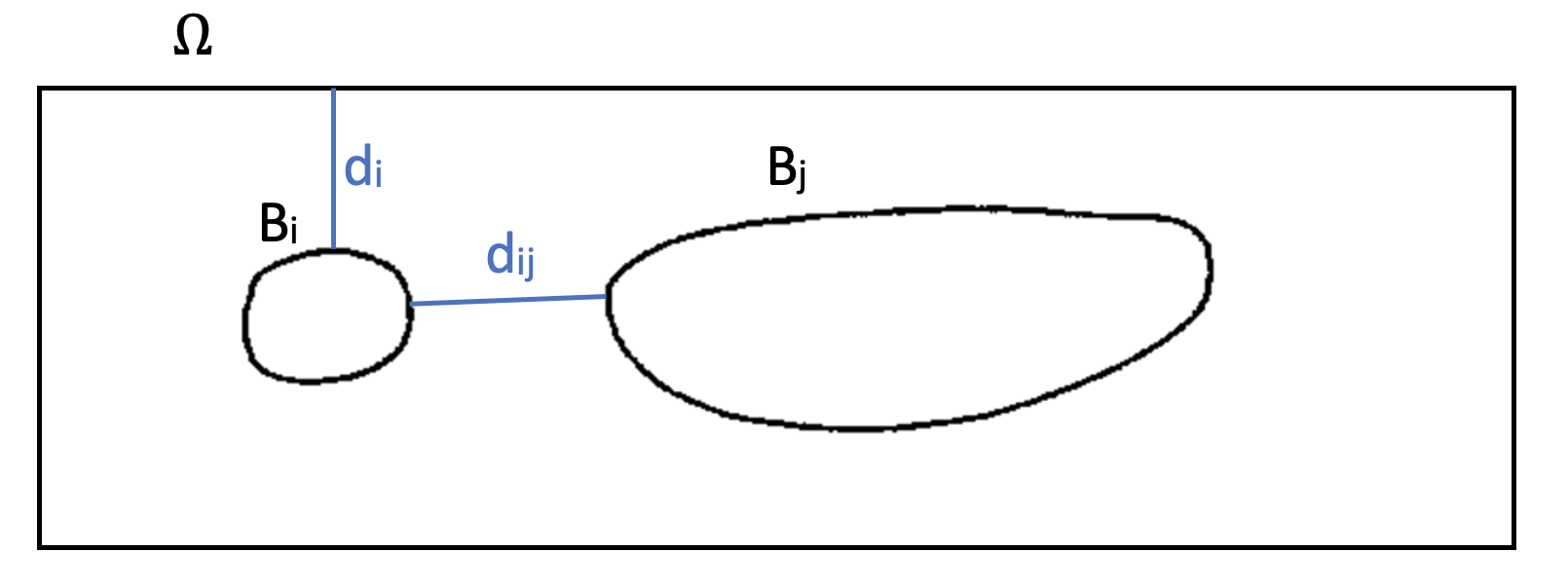
We consider two bodies $B_i$ and $B_j$, we want to find the minimal distance $d_{ij}$ between their boundaries and the minimal distance between a body and the boundary of the domain, $d_i$ for the body $B_i$. We note $D_i$ (respectively $D_j$) the distance field obtained by the Fast Marching method for the body $B_i$ (respectively $B_j$) and $D_{\Omega}$ the distance field for the fluid domain boundary. One has :

\[D_i = \left. 0 \right|_{\partial B_i} \quad \mbox{and} \quad D_j = \left. 0 \right|_{\partial B_j} \quad \mbox{and} \quad D_{\Omega} = \left. 0 \right|_{\partial \Omega}.\]

The Feel++ library contains a function, named DistanceToRange , used to retrieve the finite element fields $D_i$, $D_j$ and $D_{\Omega}$. Then, a second function, called minmax, allows to find the coordinates that minimize these fields on a boundary given as parameter. In our case, when considering the field $D_i$, it would be the boundary of the body $B_j$, so $\partial B_j$, to get $\arg\min_{x \in \partial B_j} D_i(x)$, or the boundary of the domain $\Omega$, so $\partial \Omega$, to get $\arg\min_{x \in \partial \Omega} D_i(x)$.

This function therefore allows us to determine distances by:

\[\begin{align*} d_{ij} &= ||\arg\min_{x \in \partial B_j} D_i(x) - \arg\min_{x \in \partial B_i} D_j(x)||_2 \mbox{,} \\ d_{i} &= ||\arg\min_{x \in \partial \Omega} D_i(x) - \arg\min_{x \in \partial B_i} D_{\Omega}(x)||_2 \mbox{.} \end{align*}\]

The repulsive force $|\overrightarrow{F_{ij}}|$ of the interaction between the bodies $B_i$ and $B_j$ and the repulsive force $|\overrightarrow{F_{j}}|$ of the interaction between the body $B_i$ and the domain boundary are respectively given by:

\[\begin{equation*} |\overrightarrow{F_{ij}}| = \left\{\begin{array}{rcl} 0 \;, \quad &\mbox{for }& d_{ij} > \rho , \\ \frac{1}{\epsilon}(\arg\min_{x \in \partial B_i} D_j(x) - \arg\min_{x \in \partial B_j} D_i(x))(\rho - d_{ij})^2 \;, \quad &\mbox{for }& 0 \leq d_{ij} \leq \rho . \end{array}\right.\; \end{equation*}\]

\[ \begin{equation*} |\overrightarrow{F_{i}^{W}}| = \left\{\begin{array}{rcl} 0 \;, \quad &\mbox{for }& d_{i} > \rho , \\ \frac{1}{\epsilon_W}(\arg\min_{x \in \partial B_i} D_{\Omega}(x) - \arg\min_{x \in \partial \Omega} D_i(x))(\rho - d_{i})^2 \;, \quad &\mbox{for }& 0 \leq d_{i} \leq \rho . \end{array}\right.\; \end{equation*}\]

where $\rho$ the range of the repulsion force and $\epsilon, \epsilon_W$ the stiffness parameters described in Repulsive force for spherical rigid bodies.

As the repulsion force is applied only on a thin band of thickness $\rho$ around the body, the narrow band fast marching algorithm was employed. This algorithm calculates the distance field $D_i$ up to a fixed threshold $d_{max}$.

Figure 4. Complex shapes bodies

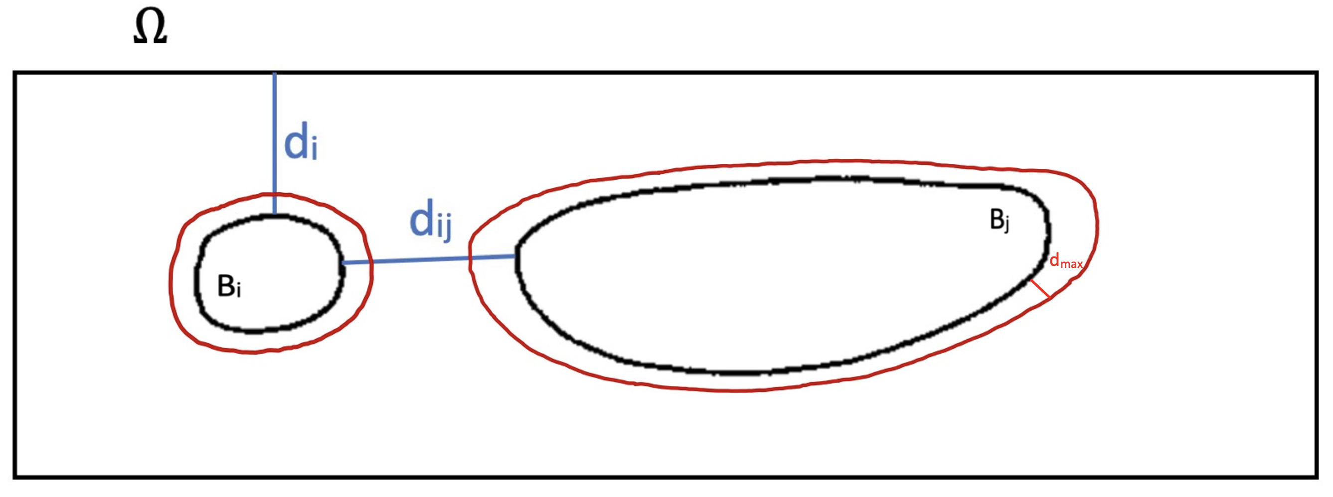
As soon as the value of the distance field is larger than the threshold value, the algorithm uses a default value $\delta$, to define the distance field. Thus, one has:

\[\begin{equation*} D_i^{NB} = \left\{\begin{array}{rcl} 0 \;, \quad &\mbox{on }& \partial B_i , \\ D_i \;, \quad &\mbox{for }& D_i \leq d_{max} ,\\ \delta\;, \quad &\mbox{elsewhere}& . \end{array}\right.\; \end{equation*}\]

To use the narrow band fast marching method, one must specify the value of $d_{max}$ in the definition of the function distanceToRange .

In the case of complex shaped bodies, one must add the torque of the collision force $F_i$ to the right-hand side of Newton’s equation describing the angular velocity $\omega_i$ of the body. Thus, this equation is written:

\[\frac{d [ R J_i R^T \omega_i ]}{d t} = M_i^e - \vec{G x_r} \times F_i ,\]

where $G$ the mass center of the body and $x_r$ the point where $F_i$ applies on the body.

Details of this Newton’s equation are given in the section Fluid-body interaction.

3. Algorithm

We will now give the different steps of this collision algorithm for complex shaped bodies. First we have a step of mesh preprocess allowing to associate the boundary markers to the bodies and the domain. The next step consists in detecting contact using the distanceToRange function. Finally, we calculate the collision force for the interactions that are taking place.

We denote by $N$ the number of bodies. The algorithm for computing the repulsion force and torque using the narrow band fast marching method is given by:

\begin{algorithm}
    \caption{Algorithm for interactions between complex shaped bodies}
    \begin{algorithmic}
    \FUNCTION{contactforce}{}

    \STATE \Comment{Read the configuration file to define:}
    \STATE $\rho$ : range of the repulsion force.
    \STATE $\epsilon, \epsilon_W$ :  stiffness parameters.

    \STATE \Comment{Mesh preprocess}

    \FOR{$1 \leq b_i \leq N$}
      \STATE \Comment{Get body markers}
      \STATE bodyMarker$_{i} \leftarrow b_i$.boundary().name()
    \ENDFOR

    \FOR{m in mesh().markerNames()}
      \IF{m not in bodyMarker}
        \STATE \Comment{Get fluid markers}
        \STATE fluidMarker$ \leftarrow $ fluidMarker.append(m)
      \ENDIF
    \ENDFOR

    \STATE \Comment{Contact Detection}

    \FOR{$0 \leq b_i \leq N$}
      \STATE \Comment{Compute distance function to $b_i$}
      \STATE $D_{i} \leftarrow $ distanceToRange(bodyMarker$_{i}$,maxdistance = $1.5*\rho$)

      \STATE \Comment{Body-body interaction}
      \FOR{$0 \leq b_j \leq N$, $b_i \neq b_j$}
        \STATE $\mbox{distBiToBj} \leftarrow $ minmax(bodyMarker$_{i}$,expr=$D_{i}$).min()
        \IF{distBiToBj $\leq \rho$}
          \STATE \Comment{Interaction $b_i$-$b_j$ is taking place}
          \STATE \Comment{Store the following values in a "DistanceParam" map: }
          \STATE Bi, Bj : body identifiers
          \STATE distBiToBj : distance between $b_i$ and $b_j$
          \STATE coordBi, coordBj : coordinates of contact point on bodyMarker$_{i}$ and bodyMarker$_{j}$
        \ENDIF
      \ENDFOR

      \STATE \Comment{Body-wall interaction}
      \FOR{$b_w$ in fluidMarker}
        \STATE $\mbox{distBiToBw} \leftarrow $ minmax(fluidMarker$_{w}$,expr=$D_{i}$).min()
        \IF{distBiToBw $\leq \rho$}
          \STATE \Comment{Interaction $b_i$-$b_w$ is taking place}
          \STATE \Comment{Store the following values in "DistanceParam" map: }
          \STATE Bi, Bw : body and boundary identifiers
          \STATE distBiToBw : distance between $b_i$ and $b_w$
          \STATE coordBi, coordBw : coordinates of contact point on bodyMarker$_{i}$ and fluidMarker$_{w}$
        \ENDIF
      \ENDFOR
    \ENDFOR

    \STATE \Comment{Compute repulsion force $F_i$ and torque $M_i$}
    \FOR{elem in DistanceParam}

      \IF{elem characterizes body-body interaction}
        \STATE activation  $ \leftarrow \rho - $elem.distBiToBj
        \STATE $G_{ij}   \leftarrow $ elem.coordBi - elem.coordBj
        \STATE $F_{ij}   \leftarrow \frac{1}{\epsilon}$ activation$^2G_{ij}$
        \STATE $F_i  \leftarrow  F_i + F_{ij} $
        \STATE $M_i  \leftarrow  (\mbox{elem.coordBi} - \mbox{Bi.massCenter()}) \times F_i$
      \ENDIF

      \IF{elem characterizes body-wall interaction}
        \STATE activation  $ \leftarrow \rho - $elem.distBiToBw
        \STATE $G_{iw} \leftarrow $ elem.coordBi - elem.coordBw
        \STATE $F_{iw} \leftarrow \frac{1}{\epsilon_W}$ activation$^2G_{iw}$
        \STATE $F_i \leftarrow F_i + F_{iw} $
        \STATE $M_i  \leftarrow  (\mbox{elem.coordBi} - \mbox{Bi.massCenter()}) \times F_i$
      \ENDIF

    \ENDFOR
    \RETURN  $F_i$, $M_i$
    \ENDFUNCTION
    \end{algorithmic}
\end{algorithm}

In this algorithm we set $d_{max} = 1.5 \rho$, where $\rho$ the safety zone thickness.

4. Test cases

4.1. Application : analytical test case to verify implementation

We will first consider three analytical test cases to check the collision algorithms.

4.1.1. Sphere - wall interaction

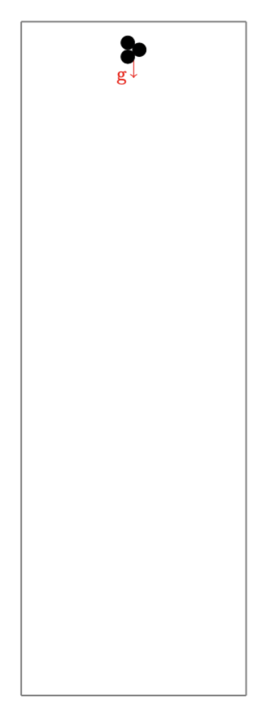
For the first test case we consider a single disk which is initially placed close to the domain boundary and falls under the effect of gravity.

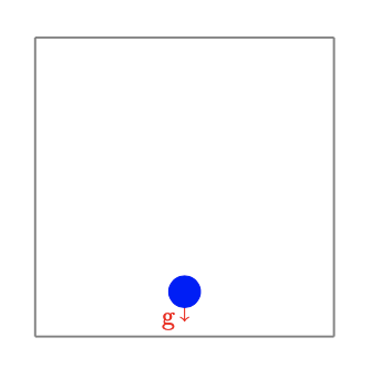
For this case we consider the following verifications:

During the iterations: the coordinate $y$ of the center of mass decreases and remains in the interval [$0,r+\rho$], where $r$ the radius of the sphere and $\rho$ the safety zone thickness.
At the end of the simulation: the translation velocity is close to $0$.
Execution time of this check: $82.81$s.

4.1.2. Square - Square interaction

The second test allows to validate the body-body collision force. The geometry consists of two squares one above the other on the same vertical line. The first square, the lower one, is initially very close to the domain boundary and the second square is falling under the effect of gravity on the first:

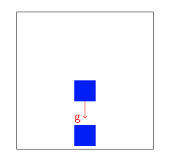
The following checks are made:

During the iterations: the vertical position of the first square remains in the interval [$0,l/2+\rho$], the one of the second square in the interval [$l,3l/2+2\rho$]. The vertical positions decrease from one iteration to another.
At the end of the simulation: the translation velocity of the two squares is close to $0$.
Execution time of this check: $79.95$s.

4.1.3. Ellipse - wall interaction

Finally, to verify that the torque of the collision force is correctly taken into account, we consider the case where an ellipse is close to the domain boundary:

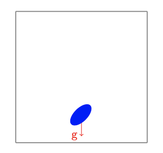
The validations that we consider are:

During the iterations: the vertical position of the ellipse decreases from one iteration to another.
At the end of the simulation: the value of the angle that the ellipse forms with the horizontal line is smaller than a given threshold. Its translation velocity is almost $0$.
Execution time of this check: $89.45$s.

4.2. Application : spherical body-body and body-bottom collisions in $2$D

For these test cases, we consider the interactions of spherical bodies and compare the execution time of the algorithm for complex shaped bodies with the two algorithms for spherical bodies described in section Repulsive force for spherical rigid bodies: the algorithm giving explicitly all the parameters (the radius of the bodies and the dimension of the box) and the method without specifying them. The purpose of these test cases is to analyze the increase in computation time for the collision algorithms when the narrow band fast marching method is used to compute either only the distance to the domain boundaries or also the distance between two bodies.

For all test cases we consider spheres of radius $0.125$ placed in a box of dimension [$0,2$] $\times$ [$0,2$]. They are placed close to the domain boundary or/and close to each other so that the collision forces are applied during the whole simulation. The spheres, of density $\rho_b = 1.01$ falls under the effect of gravity. The density of the fluid is $\rho_f = 1.0$ and its viscosity $\mu = 0.1$. The mesh size used for the simulations is equal to $h=0.01$. The simulations are realized on an interval [$0s,0.051s$] with a time step $\Delta t = 0.001s$. Thus, each simulation takes 50 iterations. The safety zone thickness is fixed at $0.03$. All parameters are listed in the following table:

Name

Description

Values

$\Omega$

Computational domain

[$0,2$]$\times$[$0,2$]

$r$

Sphere radius

$0.125$

$\rho_b$

Sphere density

$1.01$

$\rho_f$

Fluid density

$1.0$

$\mu$

Fluid viscosity

$0.1$

$\rho$

Safety zone thickness

$0.03$

$h$

Mesh size

$0.01$

$\Delta t$

Time step

$0.001$

Number of iterations

$50$

For each simulation, we will show the initial configuration of the spheres, and we will give the number of mesh elements as well as the number of executions, the execution times of the collision algorithms, and the total execution times. All simulations are executed in sequential.

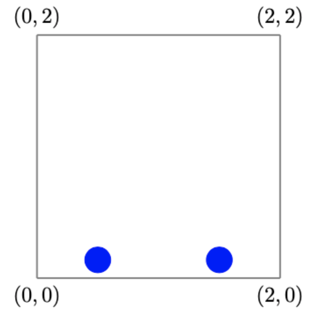
4.2.1. Case 1 : 1 sphere - bottom interaction

The initial configuration is given by:

The number of mesh elements is $93702$ and the execution times and number of executions of the collision algorithms are given by the following table:

Spherical shapes body fixed parameters

Spherical shaped body

Complex shaped body

$0.00742$s - $150$ ex.

$9.01522$s - $150$ ex.

$8.38542$s - $150$ ex.

The total execution times are as follows:

Spherical shapes body fixed parameters - total

Spherical shaped body - total

Complex shaped body - total

$104.701$s

$117.081$s

$111.828$s

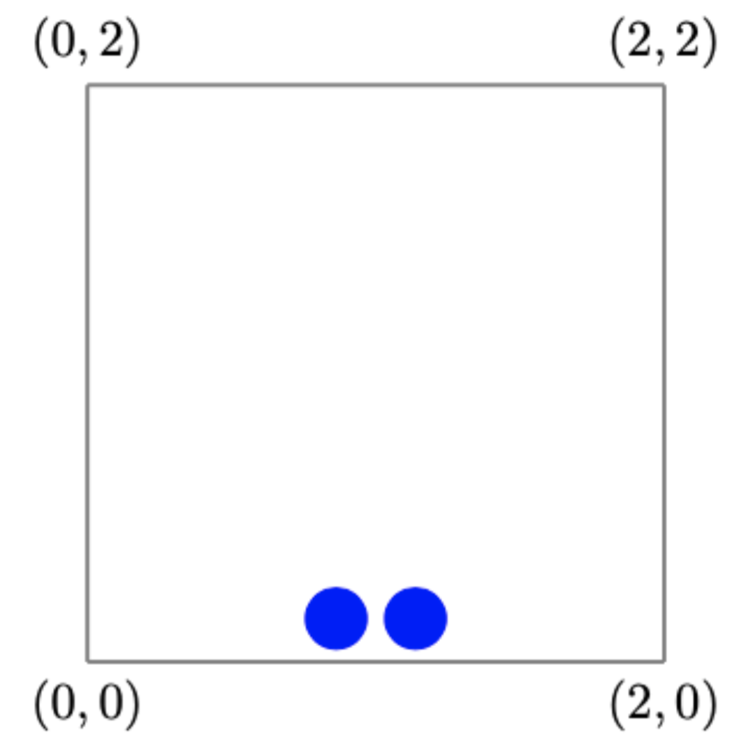
4.2.2. Case 2 : 2 spheres - bottom interaction

The number of mesh elements for the second geometry is $94104$. This geometry is visualized by:

The execution times and quantities of the collision algorithms:

Spherical shapes body fixed parameters

Spherical shaped body

Complex shaped body

$0.01226$s - $203$ ex.

$19.72834$s - $200$ ex.

$21.66329$s - $200$ ex.

and the total execution times:

Spherical shapes body fixed parameters - total

Spherical shaped body - total

Complex shaped body - total

$232.824$s

$240.804$s

$239.839$s

4.2.3. Case 3 : 2 spheres - bottom and sphere - sphere interactions

The number of elements of this mesh is fixed at $93752$. The execution data for the collision algorithms are given by:

Spherical shapes body fixed parameters

Spherical shaped body

Complex shaped body

$0.01250$s - $200$ ex.

$19.90447$s - $203$ ex.

$21.24991$s - $200$ ex.

Spherical shapes body fixed parameters - total

Spherical shaped body - total

Complex shaped body - total

$199.054$s

$224.672$s

$217.893$s

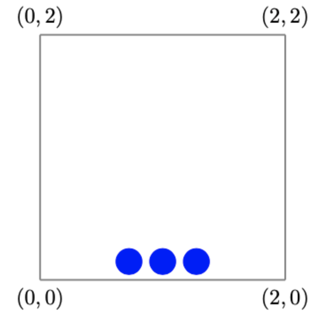
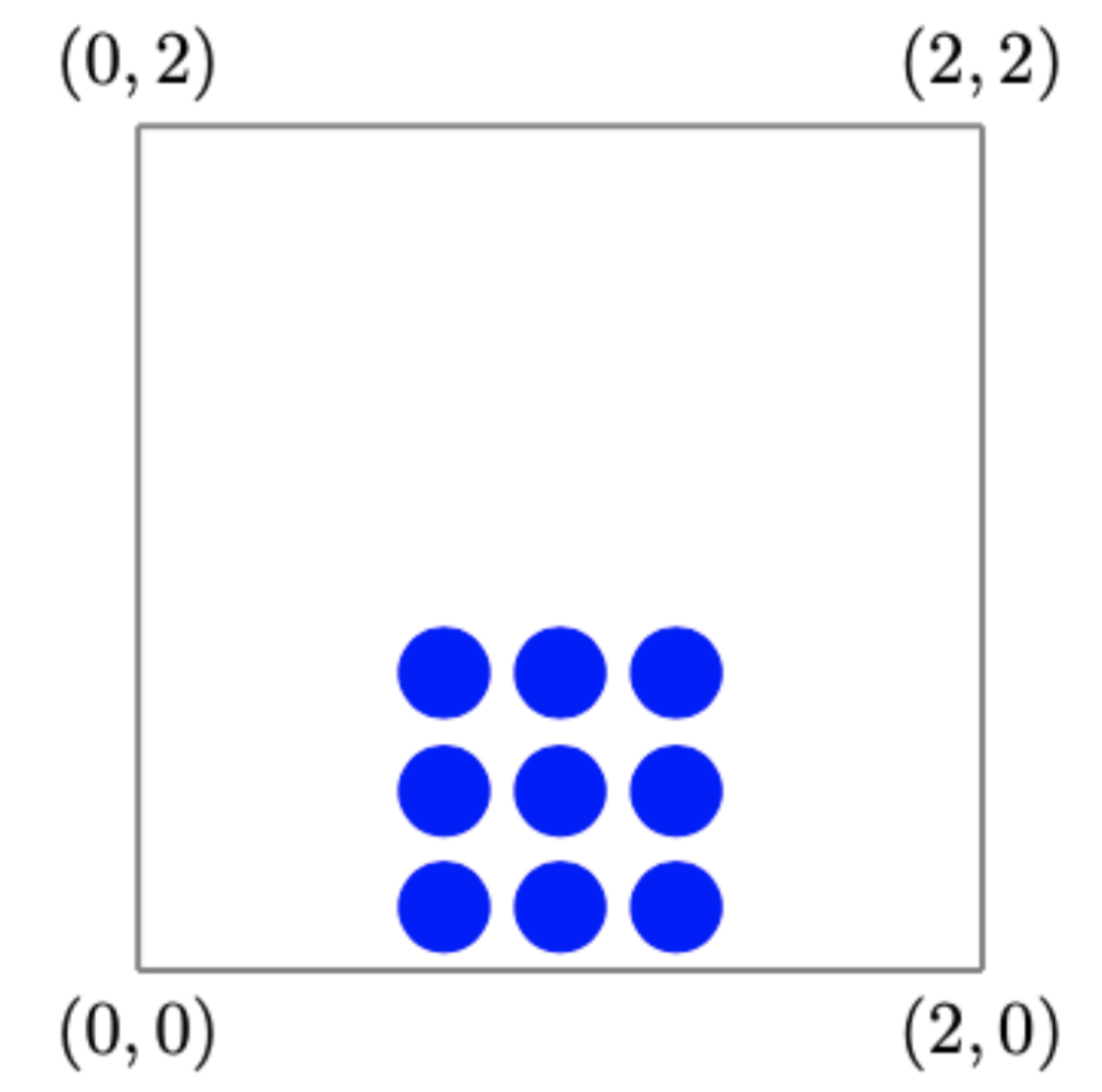
4.2.4. Case 4 : 3 spheres interactions

The initial configuration, containing $93776$ mesh elements, is given by the following figure:

The number of executions and the execution times of the collision algorithms is given by:

Spherical shapes body fixed parameters

Spherical shaped body

Complex shaped body

$0.01509$s - $200$ ex.

$26.77877$s - $200$ ex.

$33.05940$s - $203$ ex.

The total execution times are stored in this table:

Spherical shapes body fixed parameters - total

Spherical shaped body - total

Complex shaped body - total

$168.789$s

$203.657$s

$210.080$s

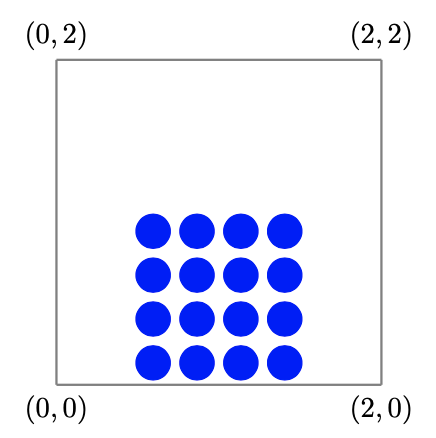
4.2.5. Case 5 : 6 spheres interactions

The next geometry is visualized by:

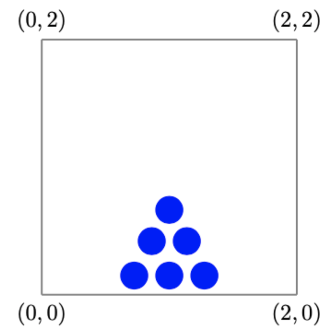
The number of mesh elements of this geometry is $94576$. The following tables show the execution times and quantities:

Spherical shapes body fixed parameters

Spherical shaped body

Complex shaped body

$0.01694$s - $200$ ex.

$41.33335$s - $206$ ex.

$73.74359$s - $203$ ex.

and the total execution times:

Spherical shapes body fixed parameters - total

Spherical shaped body - total

Complex shaped body - total

$244.922$s

$301.589$s

$331.433$s

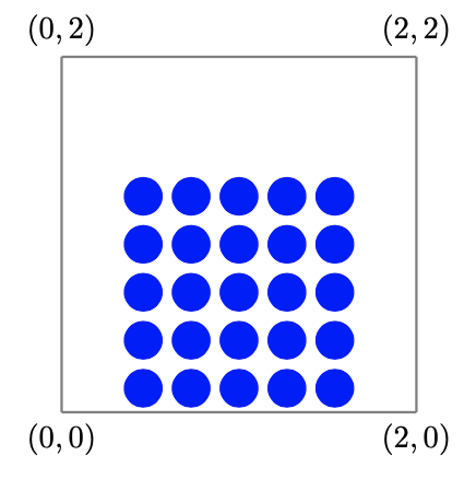
4.2.6. Case 6 : 9 spheres interactions

For this test case we use the following configuration, with $95348$ mesh elements:

Once again the execution data are given by the two tables:

Spherical shapes body fixed parameters

Spherical shaped body

Complex shaped body

$0.02529$s - $200$ ex.

$52.8046$s - $200$ ex.

$118.6058$s - $200$ ex.

Spherical shapes body fixed parameters - total

Spherical shaped body - total

Complex shaped body - total

$339.310$s

$416.791$s

$485.259$s

4.2.7. Case 7 : 16 spheres interactions

The number of mesh elements is fixed at $95766$. The execution quantities for the collision algorithms are given by:

Spherical shapes body fixed parameters

Spherical shaped body

Complex shaped body

$0.0657$s - $350$ ex.

$95.5223$s - $200$ ex.

$369.1102$s - $257$ ex.

Spherical shapes body fixed parameters - total

Spherical shaped body - total

Complex shaped body - total

$630.987$s

$694.680$s

$1004.872$s

4.2.8. Case 8 : 25 spheres interactions

For the last test case we consider the following geometry:

containig $96750$ mesh elements.

The execution times are given by the following two tables:

Spherical shapes body fixed parameters

Spherical shaped body

Complex shaped body

$0.10089$s - $344$ ex.

$159.7139$s - $203$ ex.

$1041.908$s - $311$ ex.

Spherical shapes body fixed parameters - total

Spherical shaped body - total

Complex shaped body - total

$963.623$s

$1104.613$s

$2072.229$s

All these results show that the execution time for the algorithms using the fast marching method to compute distances are much higher than the direct computation when the number of bodies increases. However, the execution times remain reasonable knowing that the execution has been done sequentially.

4.3. Application : bounding sphere in $2$D

The execution time analysis of the narrow band approach in $2$D and $3$D have shown that it is influenced by the size of the geometry on which the approach is applied. This observation leads us to investigate this influence in simulations of collision between bodies.

First, we consider spherical bodies. We generate artificial spheres bounding our bodies. The narrow band approach is applied on these artificial bounding spheres. We vary the radius $r$ of each bounding sphere to compare the execution times, $r = 2.5\rho, 3\rho$ or $r = 4\rho$, where $\rho$ the range of the collision force. For these tests, we consider the same configurations with the same parameters as for the tests of the previous part, but taking into account only the interbody collisions.

For the configuration of nine bodies, we compare the execution times for different bounding sphere radii with the case where one applies the narrow band approach on the whole domain. The simulations are run sequentially.

Bounding sphere radius

Execution time for collision algorithm

Entire domain

$0.241$s - $200$ executions

$r = 4\rho$

$0.312$s - $200$ executions

$r = 3\rho$

$0.294$s - $200$ executions

$r = 2.5\rho$

$0.292$s - $200$ executions

We can observe that the execution time decreases when the radius of the bounding spheres decreases. However, the time remains higher than the time needed when applying the narrow band approach on the whole domain. As this should not be the case, we explain it by the cost necessary to define the mesh of the bounding sphere and to impose that the narrow band method is only applied on this reduced region.

4.4. Application : rigid ellipse - bottom collision in $2$D

For this test case, we consider the interaction between an elliptic rigid body and the wall. At time $t=0$ the ellipse, placed vertically in a channel, and the fluid are at rest. Then the body falls under the effect of gravity to the bottom of the channel. The fluid, rigid body and collision parameters are listed in the following table:

Name

Description

Values

$\Omega$

Computational domain

[$0,2$]$\times$[$0,6$]

$a,b$

Ellipse long and short axis

$0.5$, $0.25$

$O$

Ellipse initial center

($1,4$)

$\rho_e$

Ellipse density

$1.25$

$\rho_f$

Fluid density

$1.0$

$\mu$

Fluid viscosity

$0.1$

$\rho$

Safety zone thickness

$0.03125$

$\epsilon_W$

Stiffness parameter for particle - wall collision

$0.00001$

$h$

Mesh size

$0.03125$

$\Delta t$

Time step

$0.001$

In order to show the trajectory of the ellipse, we show snapshots at different time instants as well as its position and its translation velocity over time.

Figure 5. Position of ellipse

The next graphs show that the ellipse is rotating until it touches the bottom. Its large side becomes horizontal.

This test case has already been performed in literature [Collision_simulations]. We do not obtain the exact same results because of the different approaches of resolution and modeling of collisions.

4.5. Validation : rigid ellipse - wall collision in $2$D

We consider again an ellipse which falls under the effect of gravity in a channel of infinite length. The channel is thin, so that the ellipse does not only collide with the bottom but also with the right and left walls. This simulation is presented in the article [Collision_ellipticalParticle]

The parameters are defined by:

Name

Description

Values

$L$

Domain width

$\frac{16}{130}$

$a,b$

Ellipse long and short axis

$0.1$, $0.05$

$\theta$

Ellipse initial angle

$\frac{\pi}{3}$

$\rho_e$

Ellipse density

$1.35$

$\rho_f$

Fluid density

$1.195$

$\mu$

Fluid viscosity

$0.305$

$\rho$

Safety zone thickness

$0.05$

$\epsilon_W$

Stiffness parameter for particle - wall collision

$0.00001$

$h$

Mesh size

$0.001$

$\Delta t$

Time step

$0.001$

The following graph compares our results with those of the literature. At the beginning the ellipse oscillates between the two walls. Then, after reaching a horizontal position, the ellipse starts to make rotations around a single wall, shown in the video. In our case, it performs these rotations close to the left wall, but in the article the rotations are made close to the right wall. This results from the differences in the collision model and the numerical resolution techniques.

When we consider for the results of the literature the symmetrical graphs for the rotations, we can observe that our results are similar. This test case allows us to validate our implementation.

The video of the simulation is given by:

4.6. Application : tripole-like rigid body - wall collision in $2$D

We continue by considering the same simulation but instead of an ellipse we use a non-convex tripole-like rigid body. The simulation is presented in [Collision_simulations]. The initial geometry is given by:

All the parameters are defined as follows:

Name

Description

Values

$\Omega$

Computational domain

[$0,2$]$\times$[$0,12$]

$O$

Body initial center

($1,11.5$)

$d$

Circle diameter

$0.25$

$\rho_e$

Body density

$1.25$

$\rho_f$

Fluid density

$1.0$

$\mu$

Fluid viscosity

$0.01$

$\rho$

Safety zone thickness

$0.03125$

$\epsilon_W$

Stiffness parmeter for particle-wall collision

$0.0000000125$

$h$

Mesh size

$0.03125$

$\Delta t$

Time step

$0.001$

The motion of the body is shown in the following video:

We can observe that the collision algorithm also allows to model the interactions between this non-convex body and the wall. The body rotates under the effect of gravity and collision forces until it reaches horizontally, thus with two circles, the bottom of the box.

4.7. Application : particle suspension in a $2$D symmetric stenotic artery

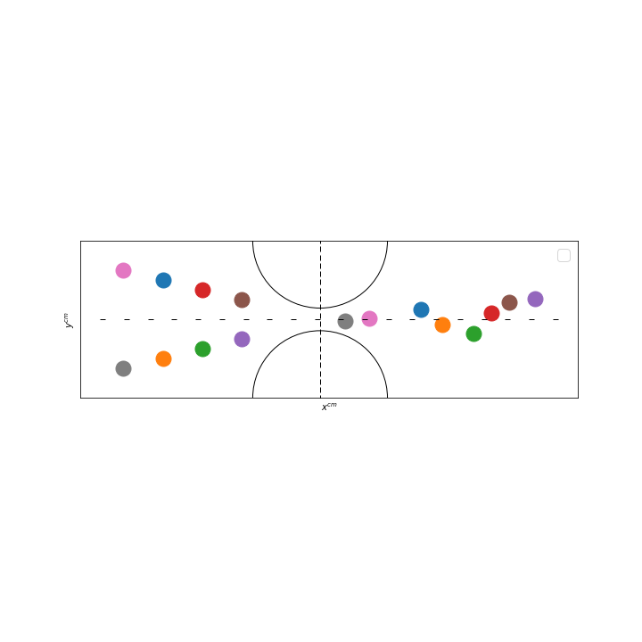
In this test case we simulate the particle suspension in a $2$D symmetric stenotic artery, presented in references [Wu_Shu] and [Stenotic_artery]. As the geometry is complex, this simulation allows to test the collision algorithms on non-rectangular domains. The geometry is given by the following figure:

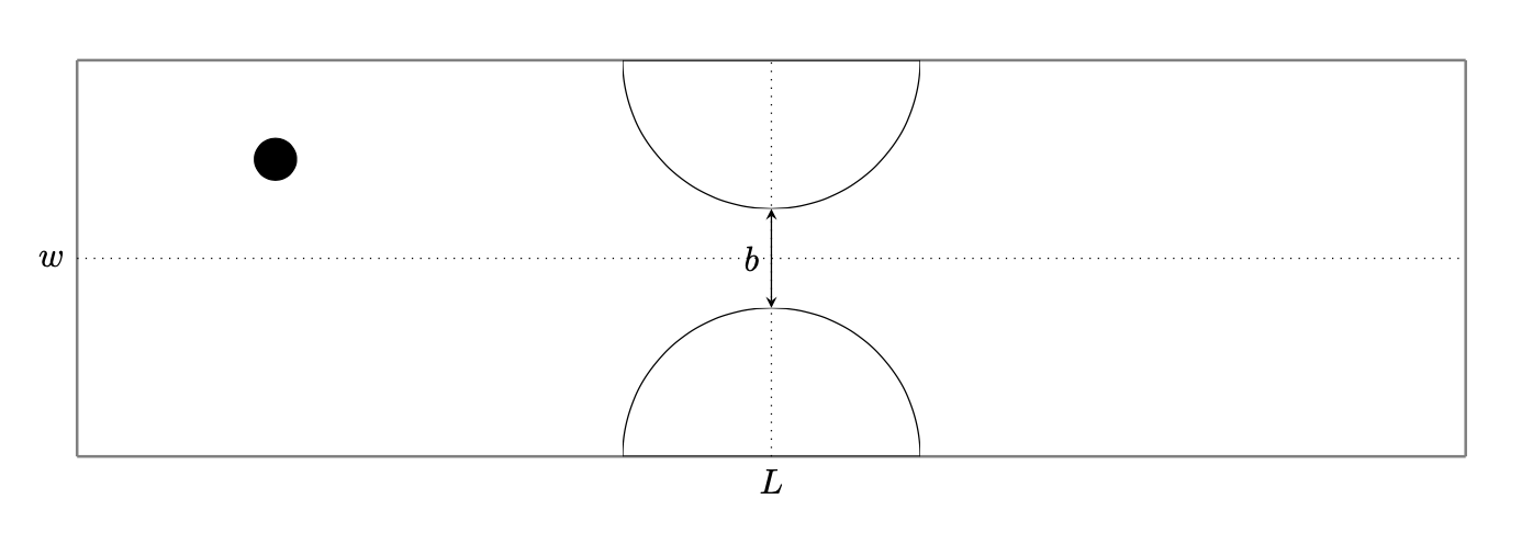
Both fluid and particles are initially at rest. The particles move under the effect of hydrodynamic forces due to a pressure difference between the inlet and outlet. The dotted line in the figure represents the centerlines. The parameters are defined by:

Name

Description

Values

$L$

Channel length

$32d$

$w$

Channel width

$8d$

$d$

Particle diameter

$8.5 * 10^{-4}$

$b$

Stenosis throat width

$1.75d$

$\mu$

Fluid viscosity

$0.01$

$\rho_f$

Fluid density

$1$

$\rho_p$

Particle density

$1$

$\Delta p$

Pressure difference

$541$

$h$

Mesh size

$0.0000607$

$\Delta t$

Time step

$0.00001$

$\rho$

Width of collision zone

$0.0003$

$\epsilon$

Stiffness parmeter for particle-particle collision

$0.00000000001$

$\epsilon_W$

Stiffness parmeter for particle-wall collision

$0.0000000000075$

We consider simulations, with one, two or several particles.

4.7.1. Single particle in a symmetric stenotic artery

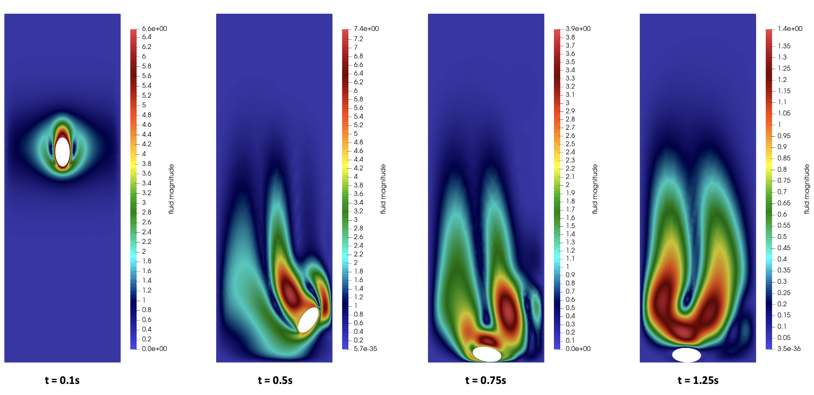
The single particle is initially centered at $2d$ above and $8d$ left to the centerline. By showing its position over time we can observe that the particle approaches the centerline when it gets near and across the protuberance. Once passed, it orients itself upwards:

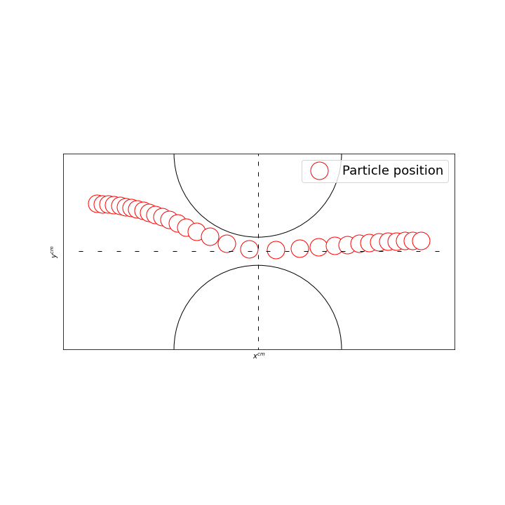
The horizontal velocity $U_x$ of the particle in the channel is about $U_x = 0.85$. When it passes the stenosis throat, the velocity is approximately $U_X = 4.15$, thus $5$ times higher.

The observations are close to the results of the literature. We do not use exactly the same configuration and collision force, thus the velocity and motion of the particle after passing the protuberance are slightly different.

4.7.2. Two particles in a symmetric stenotic artery

At $t=0$, two particles are located asymmetrically with respect to the center. Both particles are placed at a distance $8d$ at the left of the vertical centerline. The upper particle is $2d + s$ above and the lower one $2d$ below the horizontal line. The parameter $s$ is fixed at $s = \frac{d}{4000}$. Due to this slight asymmetry, the two particles will pass the stenotic throat.

We will first plot the position of the two particles over time, before analyzing in detail the moment when the two particles cross the throat.

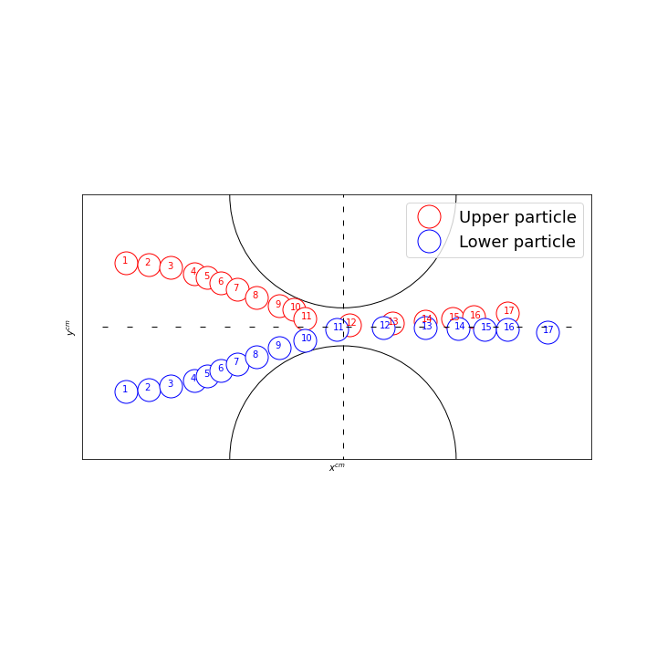
The particles move side by side, represented by the snapshot $1-9$, until they are near the stenotic throat, snapshot $10$. This latter indicates that the upper particle stops and moves back to allow the lower particle, that keeps moving, to pass the throat. Once passed, the upper particle changes direction and follows the first particle through the artery, shown by snapshot $11-17$.

To analyze what happens at the time of snapshot $10$, we will show the horizontal position of the particles over time shortly before and after this moment.

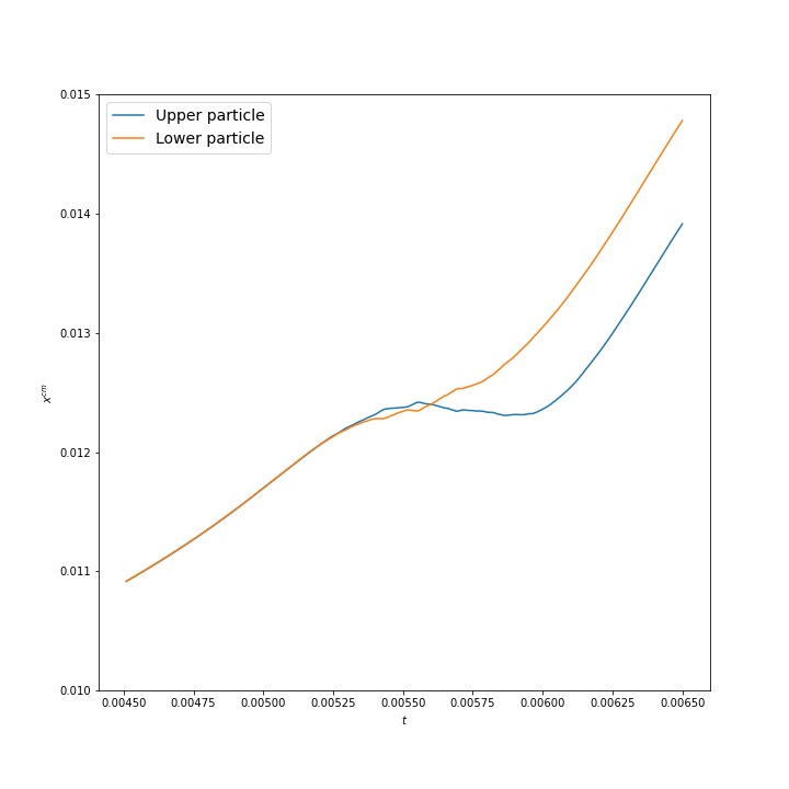
This plot, illustrating the horizontal position of the two particles, corresponds well to the observations of the first figure.

The motion of the particles is shown in the following video:

4.7.3. Many particles in a symmetric stenotic artery

Finally, we consider several particles initially placed asymmetrically in the artery. By showing the position of each of the particles for two different time instants, we can observe that they all manage to cross the throat:

References on collision models

[Glowinski] R. Glowinski, T. W. Pan, T. I. Hesla, D. D. Joseph, and J. Périaux (2000). A Fictitious Domain Approach to the Direct Numerical Simulation of Incompressible Viscous Flow past Moving Rigid Bodies: Application to Particulate Flow. Download PDF
[AIP_Advances] K. Usman, K. Walayat, R. Mahmood, et al. (2018). Analysis of solid particles falling down and interacting in a channel with sedimentation using fictitious boundary method. Download PDF
[Computers_Fluids] L. Wang, Z.L. Guo, J.C. Mi (2014). Drafting, kissing and tumbling process of two particles with different sizes. Download PDF
[Wan_Turek] Decheng Wan and Stefan Turek (2004). Direct Numerical Simulation of Particulate Flow via Multigrid FEM Techniques and the Fictitious Boundary Method. Download PDF
[Multiphase_Flow] P. Singh, T.I Hesla, D.D Joseph (2002). Distributed Lagrange multiplier method for particulate flows with collisions.
[Settling_ellipsoid] Tsorng-Whay Pan, Roland Glowinski, Giovanni P.Galdi (2001). Direct simulation of the motion of a settling ellipsoid in Newtonian fluid. Download PDF
[FMM_1] J.A. Sethian (1996). A fast marching level set method for monotonically advancing fronts.
[FMM_2] J.A. Sethian (1996). Level Set Methods and Fast Marching Methods; Evolving Interfaces in Computational Geometry, Fluid Mechanics, Computer Vision and Materials Sciene.
[FMM_3] J.A. Sethian. Level Set Methods and Fast Marching Methods.
[CollisionModel_DNS] Ramandeep Jain, Silvio Tschisgale, Jochen Fröhlich (2019). A collision model for DNS with ellipsoidal particles in viscous fluid.
[DNS_Framework] S.Tschisgale, T.Kempe and J.Fröhlich (2018). A general implicit direct forcing immersed boundary method for rigid particles.
[Wu_Shu] J.Wu, C.Shu (2009). Particulate Flow Simulation via a Boundary Condition-Enforced Immersed Boundary-Lattice Boltzmann Scheme.
[Stenotic_artery] H.Li, H.Fang, Z.Lin, S.Xu, S.Chen (2004). Lattice Boltzmann simulation on particle suspensions in a two-dimensional symmetric stenotic artery.
[Collision_simulations] L.H. Juarez, R. Glowinski, T.W. Pan (2004). Numerical Simulation of Fluid Flow with Moving and Free Boundaries. Download PDF
[Collision_ellipticalParticle] Zhenhua Xia, Kevin W. Connington, Saikiran Rapaka, Pengtao Yue, James J. Feng, Shiyi Chen (2008). Flow patterns in the sedimentation of an elliptical particle. Download PDF
[Sphere_interaction] S.M. Dash, T.S. Lee (2015). Two spheres sedimentation dynmics in a viscous liquid column.
[MMG] www.mmgtools.org/mmg-remesher-try-mmg/mmg-remesher-tutorials/mmg-remesher-mmg2d/implicit-domain-meshing.

Repulsive force for arbitrary rigid bodies

1. Tools : Fast Marching methods

1.1. Mathematical framework

1.2. Test cases in \(2\)D

1.3. Test cases in \(3\)D

2. Mathematical formulation

3. Algorithm

4. Test cases

4.1. Application : analytical test case to verify implementation

4.1.1. Sphere - wall interaction

4.1.2. Square - Square interaction

4.1.3. Ellipse - wall interaction

4.2. Application : spherical body-body and body-bottom collisions in \(2\)D

4.2.1. Case 1 : 1 sphere - bottom interaction

4.2.2. Case 2 : 2 spheres - bottom interaction

4.2.3. Case 3 : 2 spheres - bottom and sphere - sphere interactions

4.2.4. Case 4 : 3 spheres interactions

4.2.5. Case 5 : 6 spheres interactions

4.2.6. Case 6 : 9 spheres interactions

4.2.7. Case 7 : 16 spheres interactions

4.2.8. Case 8 : 25 spheres interactions

4.3. Application : bounding sphere in \(2\)D

4.4. Application : rigid ellipse - bottom collision in \(2\)D

4.5. Validation : rigid ellipse - wall collision in \(2\)D

4.6. Application : tripole-like rigid body - wall collision in \(2\)D

4.7. Application : particle suspension in a $2$D symmetric stenotic artery

4.7.1. Single particle in a symmetric stenotic artery

4.7.2. Two particles in a symmetric stenotic artery

4.7.3. Many particles in a symmetric stenotic artery

References on collision models