Collision model for DNS

The hydrodynamic forces are described by the unsteady Navier-Stokes equations for Newtonian fluid, including a coupling force to take into account the particle-fluid interaction.

The particle-fluid interaction can be visualized by the following figure, allowing also to have a global view on the different parameters:

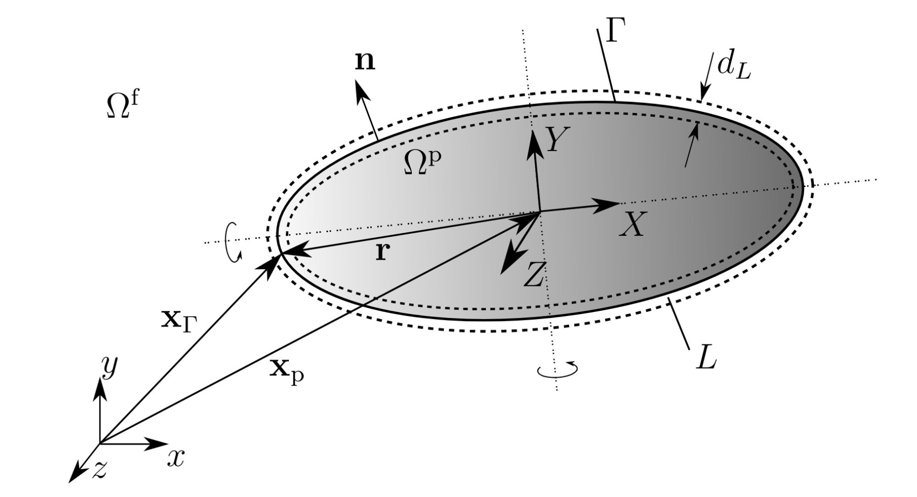
The translational velocity \(u_p\) of the particle is described by:

where \(V_p\) the volume, \(\rho_p\) the density and \(m_p\) the mass of the particle of boundary \(\Gamma\). The fluid density is denoted \(\rho_f\) and \(\tau\) is the hydrodynamic stress tensor. \(f_v\) represents the external forces applied on the fluid and \(g\) the gravity. The two terms \(f_c\) and \(f_{lub}\) correspond respectively to the collision force and the lubrication force.

The angular velocity is given in a body-fixed local frame that coincides with the principal axes of the particle. Any vector can be converted from the local frame into the global coordinate system with the rotation matrix \(\mathcal{R}\) by the transformation:

where capital letters are given in body-fixed local frame and small letters in global frame. The angular velocity \(\Omega_p\) of the particle in local frame is described by:

where \(I_p\) is the tensor of inertia. \(R\) denotes the vector of a surface point to the mass center and \(T\) the hydrodynamic stress tensor. The torque due to collision force and to lubrication force are respectively described by \(M_c\) and \(M_{lub}\).

The motion of a particle in a fluid, characterized by the Immersed Boundary Method, is given by the following discretized equation:

where \(m_L\) is the mass of the fluid layer \(L\) of width \(d_L\) and \(f_f\) the time-discrete fluid force acting on the particle, \(f_g\) the time-discrete gravitational force. The fluid layer \(L\) must be introduced to properly model the boundary conditions of the particles during their interaction with the fluid.

The angular discretized equation is defined as:

where \(I_L\) the tensor of inertia of the fluid layer \(L\) and \(M_f\) the torque due to fluid forces acting on the particle.

These two equations, better described in [DNS_Framework], are the starting point for the collision model.

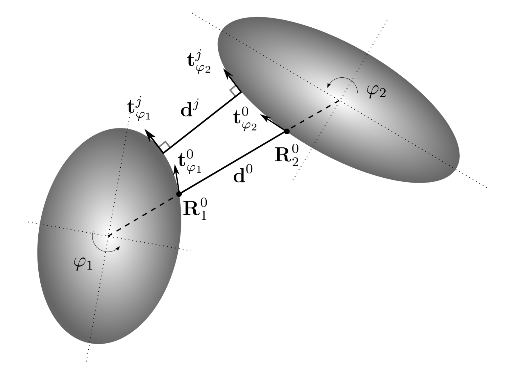
The first step of the collision model is a contact detection algorithm. The algorithm presented by the authors is iterative and does not depend on additional parameters. To better understand the computations performed during each iteration one considers the following figure:

A point on the boundary of an ellipsoidal particle, expressed in local frame, is denoted \(R = (R_X, R_Y, R_Z)^T\). The coordinates are expressed using the parametric equations of an ellipsoid:

The longest, intermediate and smallest axis of the ellipsoid are respectively denoted by \(a\), \(b\) and \(c\). \(\phi \in\)]\(-\pi,\pi\)] is the azimuthal angle and \(\varphi \in\)[\(0,\pi\)] the polar angle.

Differentiating the parametric equations in \(\phi_i\) and \(\varphi_i\) direction allow to find the vectors tangential to the boundary of the particle \(P_i\), noted \(t_{\phi_i}\) and \(t_{\varphi_i}\), located at the point \(R_i = R_i(a_i,b_i,c_i,\varphi_i,\phi_i)\). As the length of the three axis \(a_i,b_i,c_i\) remains unchanged, the coordinates of the point \(R_i\) depends only on the angles \(\phi_i\) and \(\varphi_i\).

The distance between two ellipsoids \(P_1\) and \(P_2\) is then estimated by the distance vector between \(R_1\) and \(R_2\). The minimum distance is achieved when the distance vector \(d\) is perpendicular to the tangent vectors. The idea of this algorithm is to update the two angles \(\phi_i\) and \(\varphi_i\) at each iteration until the dot products \(d \cdot t_{\phi_i}\) and \(d \cdot t_{\varphi_i}\) are smaller than a given threshold. The threshold is set to \(0.2 \Delta x\), where \(\Delta x\) the mesh size.

The formula for updating the \(\phi_i\) and \(\varphi_i\) are given by:

where \(j\) indicates the \(j\)-th iteration and \(D_{eq,i}\) the volumetrically equivalent diameter of the ellipsoid. The quantity that is added at each iteration is proportional to the dot product, which increases the rate of convergence. For the first iteration one chooses \(R_i^{0}\) in a way that the surface point is on the line that passes through the particles centers. The collision with a wall is considered as a collision with a sphere of radius \(r = 10^{12}\).

This contact detection algorithm is applied when two particles are already relatively close, they must verify:

where \(x_{p,i}\) the particle center and \(d_{lub} = 2 \Delta x\).

A collision force is applied when the surfaces of two particles are in direct contact. The starting point of this model is the moment when two ellipsoids come into contact for the first time:

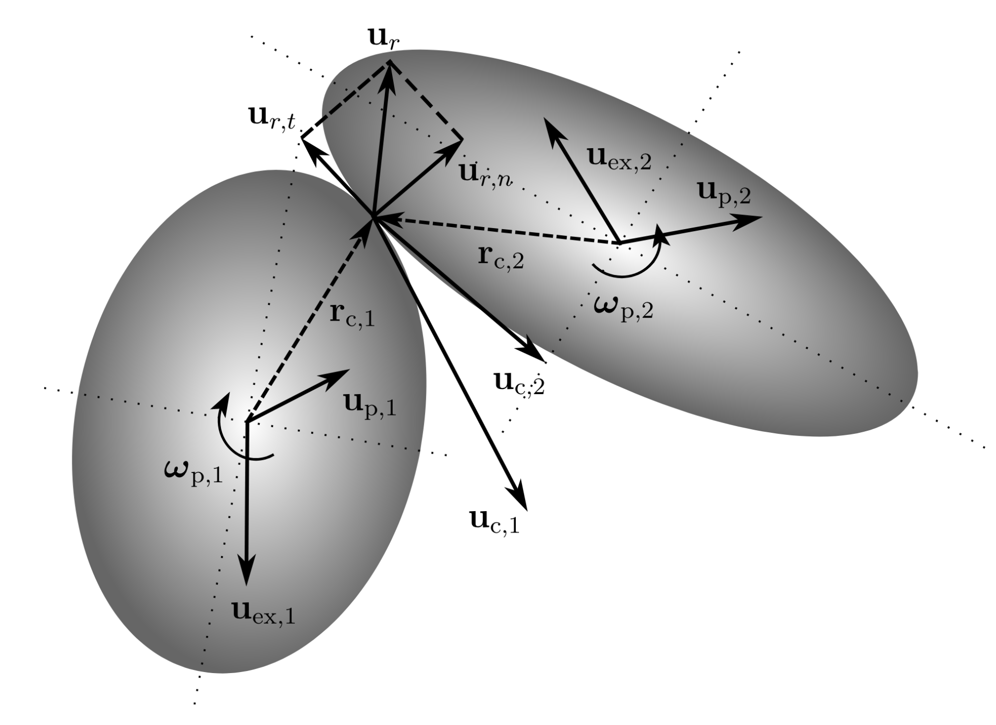
To describe the motion of the particles, influenced by the contact and described by a discrete equation, we consider here that the configuration of the figure corresponds to the discrete time level \(t^{n-1}\). In the hard-sphere approach, the collision time is very small. Thus, at the time of the first contact, the velocities of the two particles are updated while their position and orientation remain unchanged. This property allows to estimate the collision force, at each time step, by a constant value. In the following, we will detail how to determine this constant value.

To estimate the collision force, we first consider the velocity at the contact points of the two particles. At the moment after the first contact, i.e. at the discrete time level \(t^n\), the velocity at contact point \(u_c^n\) satisfies:

where \(r_c\) represents the vector between the particle center and the contact point. By replacing the translational velocity \(u_p^n\) and the angular velocity \(\omega_p^n\) by their expression described in the first paragraph, one finds for \(u_c^n\) the following formulation:

where \(u_{ex}\) represents the velocity due to external forces (hydrodynamic, gravitational and lubrication forces). This quantity can be computed at discrete time level \(t^{n-1}\). \(p_c = \Delta t f_c\) and \(l_c = \Delta t m_c = r_c \times p_c\) are the linear and angular momentum due to collision. The relationship between the latter allows us to rewrite the expression of \(u_c^n\):

where \(K\) a symmetric system matrix.

Let’s consider this expression for the two colliding particles. \(p_c\) has same magnitude for both particles, but is directed in opposite direction:

Therefore, the value of \(p_c\) can be determined by subtracting the equations:

One have \(u_r^n = u_{c,2}^n - u_{c,1}^n\) the relative velocity at contact point.

This formulation still contains an unknown quantity, \(u_r^n\), which the authors determined with the Poisson hypothesis. \(u_r^n\) is decomposed into its normal and tangential quantity \(u_{r}^n = u_{r,n}^n + u_{r,t}^n \). These quantities are expressed by:

where \(e_{d,n}, e_{d,t}\) the dry and tangential coefficient of restitution, \(t\) is defined as \(t = \frac{u_r^{n-1} - u_{r,n}^{n-1}}{|u_r^{n-1} - u_{r,n}^{n-1}|}\).

If the particles stick after the contact, the tangential coefficient of restitution \(e_{d,t} = 0\) is known and thus one can compute \(u_r^n\). The change in relative velocity during a collision is:

The expression for \(p_c\) becomes:

One can determine \(p_c\) and thus the value of the collision force and torque in the case where the two particles stick after the contact.

When two particles slide after contact, which is the case when:

where \(\mu_s\) the static coefficient of friction, \(p_c\) has to be modified to allow sliding in tangential direction. Using the Coulomb law of friction, one can express the linear momentum for two particles sliding after contact by the following equation:

where \(\mu_k\) the kinetic coefficient of friction.

To ensure that the hydrodynamic forces are also resolved in the case where two particles are very close, short time before and after contact, the authors consider a lubrication model. The model used applies a constant force when the distance \(d\) is smaller than a fixed parameter \(d_{lub} = 2 \Delta x\). In the case of spherical particles, this force depends on the Stokes number, the radii of the particles, the distance \(d_{lub}\), the viscosity of the fluid and the normal relative velocity:

The function \(k(St_r)\), where \(St_r\) the relative Stokes number:

is determined by a Gauss function:

where \(\alpha=125\), \(\sigma=100\).

This lubrication model can be extended to non-spherical particles. To apply this lubrication model to the case of ellipsoids, the authors use an expression based on the Gaussian curvature of the ellipsoidal particles at the contact point \(R\). The radii of the spheres of the first model are replaced by the radii of Gaussian curvature, defined by:

where \(G\) the Gaussian curvature at point \((x,y,z)\),

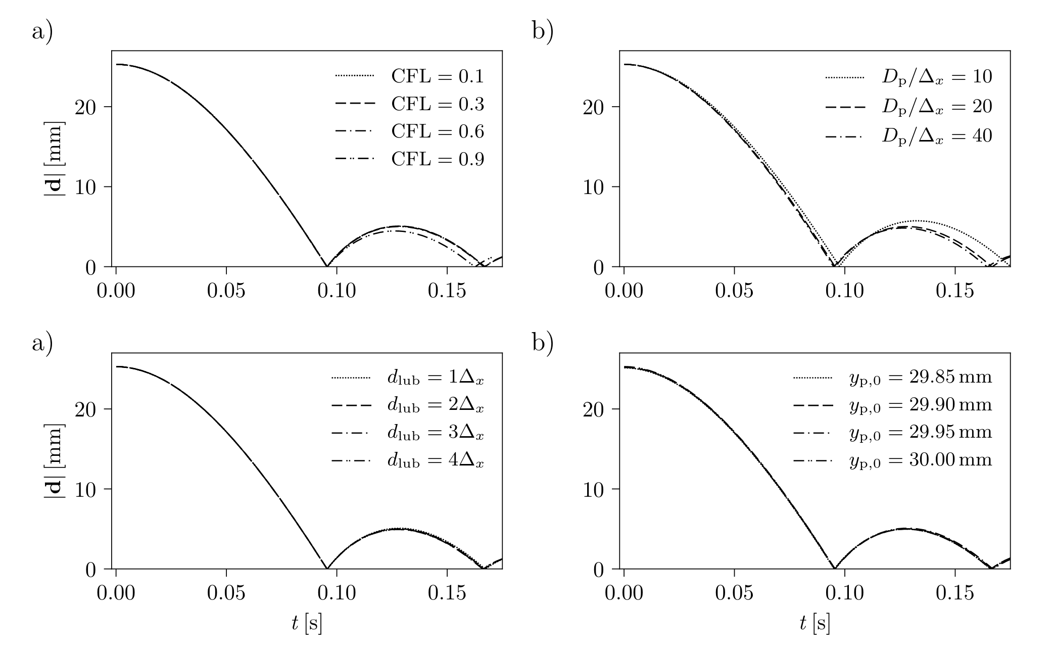
The authors analyzed the sensitivity of the collision model to various parameters, such as the CFL number, the mesh size, the width of the lubrication region \(d_{lub}\) and the initial position of a falling particle. For this analysis they consider a particle-wall interaction. During each simulation, they vary the value of only one of the four parameters and compare the resulting trajectory with a reference trajectory. We will briefly detail the conclusions that can be taken from this analysis:

The authors have considered different benchmarks to validate their collision model. For these validations they used collisions between spherical particles and the wall.

Validation 1 : Normal collision of a spherical particle with a wall

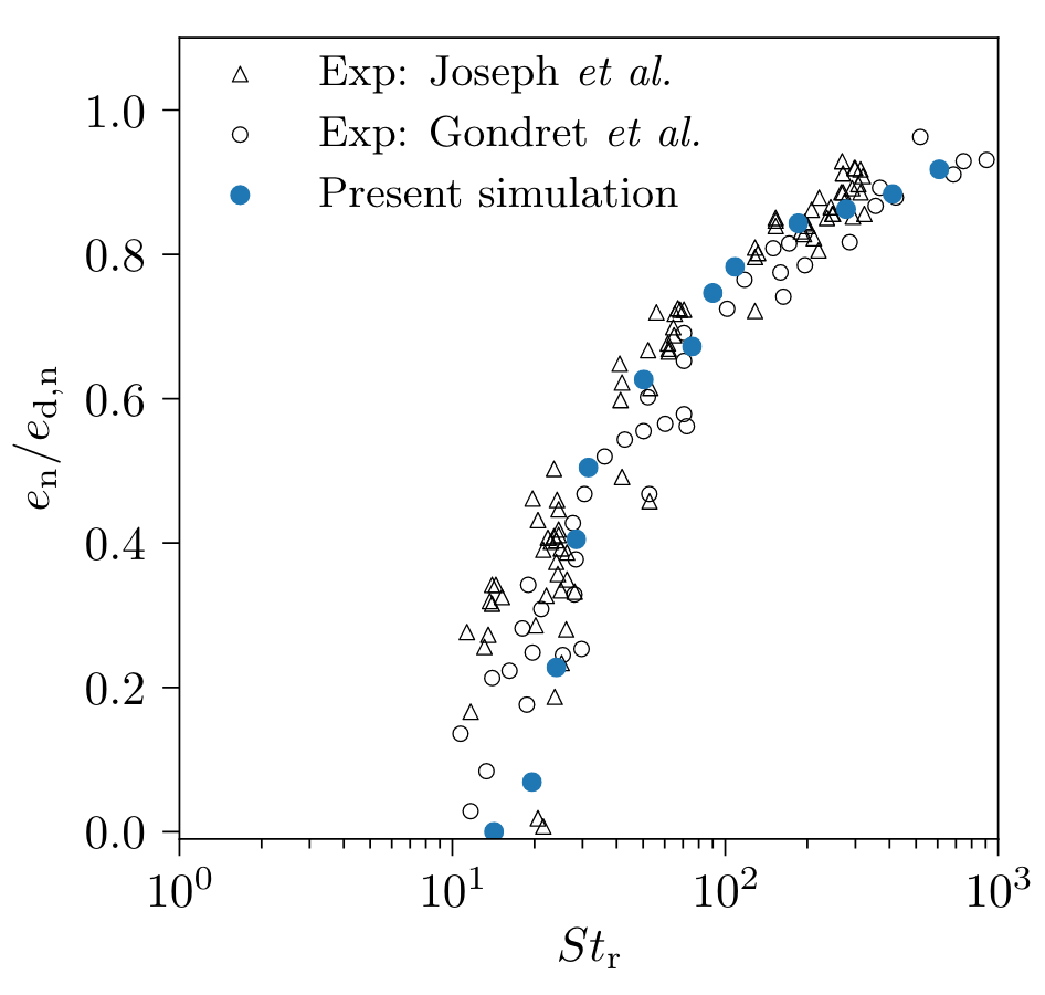
The authors analyze the influence of the relative Stokes number on the restitution coefficient for normal collision:

where \(u_{p,n,out},u_{p,n,in}\) the particle normal velocities before and after the lubrication zone. This parameter gives information on the particle’s rebound trajectory. More the normalized coefficient of restitution is close to 1, the greater will be the rebound.

The following plot shows that the normalized coefficient is increasing as a function of the relative Stokes number. Moreover, the results are consistent with the results of the literature.

Validation 2 : Oblique collision of a spherical particle with a wall

The authors compare the rebound angle to the impact angle of a particle that collides with the wall at an angle \(\phi_{in}\). Once again, the authors get the results of the literature.

The purpose of the test cases is to analyze the influence of the axis length and the initial orientation of the particles on the rebound trajectory.

Result 1 : Oblique collisions of ellipsoidal particles

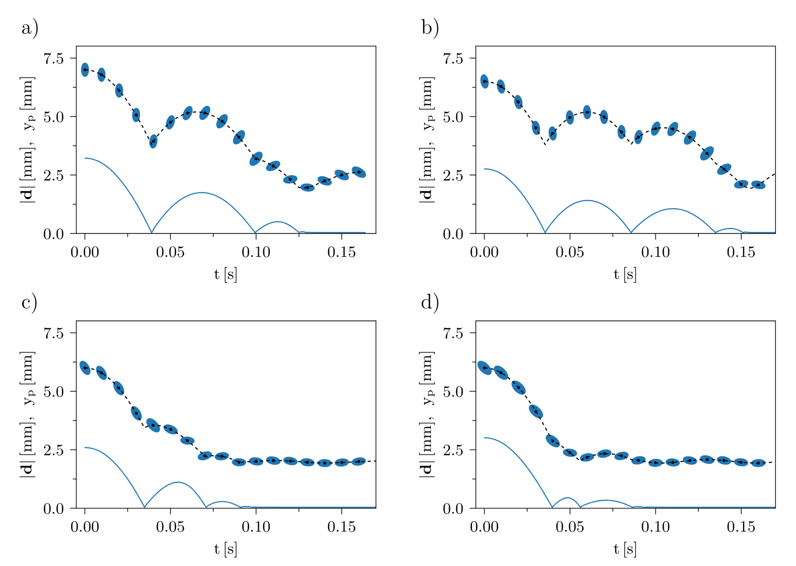
The authors analyze these rebound trajectories for different initial orientation of the ellipsoidal particle. The graphs show the results obtained for four different angles varying between \(frac{\pi}{2}\) and \(\frac{\pi}{4}\). The solid lines represent the distance between the particle surface and the wall and the dotted lines represent the position and orientation of the particle. The rebound trajectory is damped more and more as the orientation angle approaches \(\frac{\pi}{4}\).

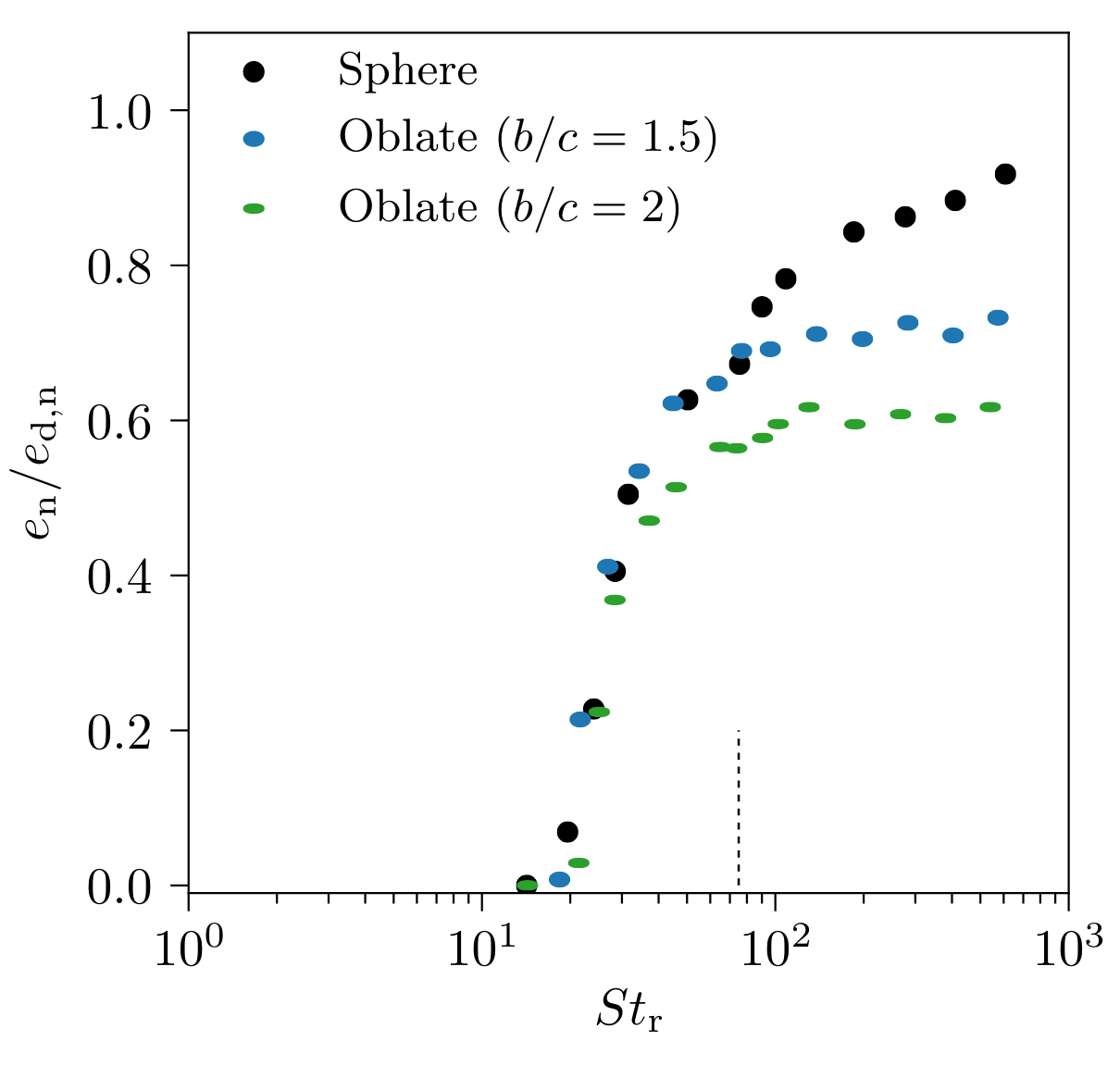
Result 2 : Normal collisions of oblate particles with a wall

The rebound trajectories of ellipsoidal particles with different ratio of axis length have been studied. The following figure shows that the maximum value of the normalized coefficient of restitution decreases when this ratio increases. This is due to the fact that the magnitude of the lubrication force increases when the particles get more flattened and therefore when the radius of Gaussian curvature increases.

The authors cited several recent references on other collision models:

Soft sphere collision model:

Collision model for complex shaped particles:

Hertzian contact theory:

Adaptive collision model:

Multi-collision model: