 .pdf
.pdf
Summary of Articles
In these articles, the linked three spheres swimmer has been studied. The swimmer consists of three spheres of radius \(R\) and linked by rigid rods whose lengths can change. The lateral spheres are separated from the central one by a distance of \(D\).
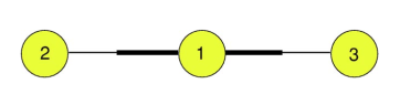
1. Article 1 : Simple swimmer at low Reynolds number: Three linked spheres
In this article [Najafi_2004], The authors have proposed a nonreciprocal motion (shown in figure below) that guarantees the self propolsion of the swimmer. The complete cycle of the motion is described as follow :
The cycle consists of four consecutive time-reversal breaking stages:
-
a) The left arm decreases its length with a constant relative velocity.
-
b) The right arm decreases its length with the same velocity.
-
c) The left arm opens up to its original length.
-
d) The right arm elongates to its original size.
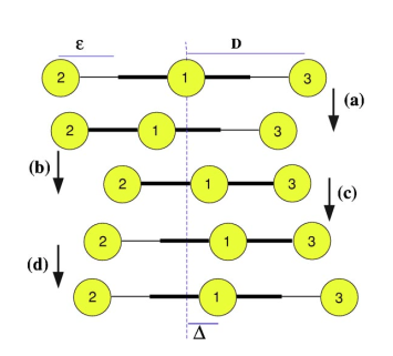
By repeating the above cycle continuously, we can get a net translation of the swimmer.
The general equation describing the hydrodynamics of low Reynolds number flow is the Stokes equation given by :
\[ \begin{equation} \mu\nabla^{2} u - \nabla p = 0 \end{equation}\]
\[ \begin{equation} \nabla . u = 0, \end{equation} \]
where \(u\) and \(p\) are the velocity and the presssure fields in the medium.
For the boundary conditions, at infinity the velocity is equal to zero, and on the spheres surface, there is a no slip boundary conditions :
\[ u_r = V_i\qquad on\; the\; spheres,\]
where \(V_i\) is the spheres velocity vector inside the fluid.
By solving the equations above, we obtain the fluid velocity in the medium and the stress tensor that will give us the forces on the shperes. The linearity of the Stokes equation and the stress tensor (with respect to the velocity field) gives the following equation :
\[ V_i = \sum_{j=1}^{3}\mathcal{H}_{ij}.\text{F}_j,\]
where \(\text{F}_j\) are the forces acting on the spheres and \(\mathcal{H}_{ij}\) is the symmetric Oseen tensor.
Including the fact that there are no external forces, we have the equation :
\[ \sum_{j=1}^{3}\text{F}_j=0.\]
Since we want to determine the dynamics of the spheres, we can solve the last two equations instead of the Stokes equation. The Oseen tensor form is given by :
\[ \mathcal{H}_{ij}= \frac{1}{6\pi\mu R}[A_{ij}(\lambda)\hat{\mathbf{n}}\hat{n} +B_{ij}(\lambda)(\text{I} - \hat{\mathbf{n}}\hat{n})], \]
where \(\lambda=\displaystyle{\frac{R}{x_i-x_j}}\) and :
\[ A_{ij} = \begin{cases} 1+\mathit{O}(\lambda^4), & i=j \\ \displaystyle{\frac{3}{2}}\lambda_{ij}+\mathit{O}(\lambda^3), & i\neq j \end{cases} \] and
\[ B_{ij} = \begin{cases} 1+\mathit{O}(\lambda^4), & i=j \\ \displaystyle{\frac{3}{4}}\lambda_{ij}+\mathit{O}(\lambda^3), & i\neq j. \end{cases} \]
As numerical example, for \(D=10 R\) and \(\varepsilon = 4R\), here are the displacements of the middle sphere after each stroke :
-
a) It swims in the \(-x\) direction by an amount of \(1.35 R\).
-
b) It swims a distance of \(1.44 R\) in the positive direction.
-
c) It swims again a distance of \(1.44 R\) in the positive direction.
-
d) It moves back by the distance of \(1.35 R\).
After this cycle, the sphere is displaced forward by an amount of \(0.16 R\). Repeating this cycle of motion makes the swimmer moves in the desired direction.
2. Article 2 : Self-learning how to swim at low Reynolds number
In this article, a new approach to designe low Reynolds number swimmers with machine learning is presented. The idea is to exploite reinforcement learning so the swimmer can develop its own propulsion strategy based on the interactions with the surrounding medium instead of specifiying any locomotory gaits.
Here, the swimmer have to learn how to act by interacting with surrounding fluid. For a given state \(s_n\) of the swimmer, in the n-th learning step the swimmer can extend or contract one of its rods (action \(a_n\)) to transform from the current state to a new state. This displacement of the swimmer provides a reward \(r_n\) to measure the immediate success of the action.
The experiences gained by the swimmer will be stored in a \(\mathit{Q}\)-matrix, \(\mathit{Q}(s_n,a_n)\). A classical \(\mathit{Q}\)-learning algorithm is used to elucidate the machine learning approach.
The \(\mathit{Q}\)-matrix is updated after each step as :
\[ \mathit{Q}(s_n,a_n)\leftarrow\mathit{Q}(s_n,a_n)+\alpha[r_n + \gamma\; \max_{a_n+1}\mathit{Q}(s_{n+1},a_{n+1})-\mathit{Q}(s_n,a_n) ], \] where \(0\leq\alpha\leq1\) is the learning rate and \(0\leq\gamma\leq1\) is the weight.
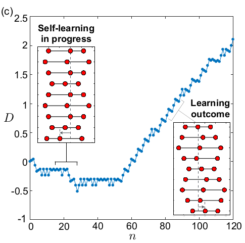
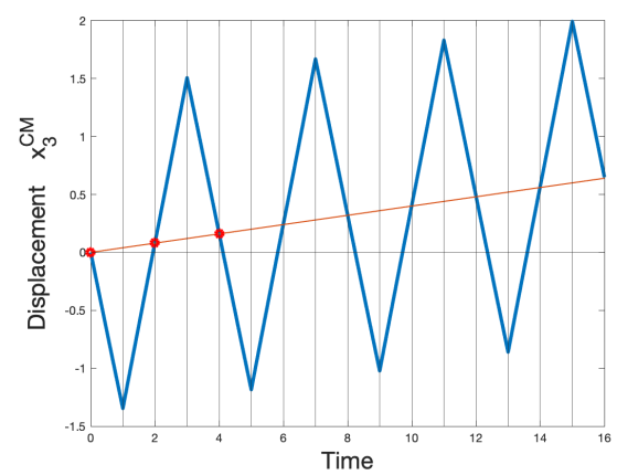
This figure shows the process of the self-learning of the swimer, the cumulative displacement of the swimmer advances over learning steps. The swimmer struggles to propel but after accumulating sufficient knowledge (almost 60 steps), the swimmer develops its own effective manner of swimmming and repeats it over time.
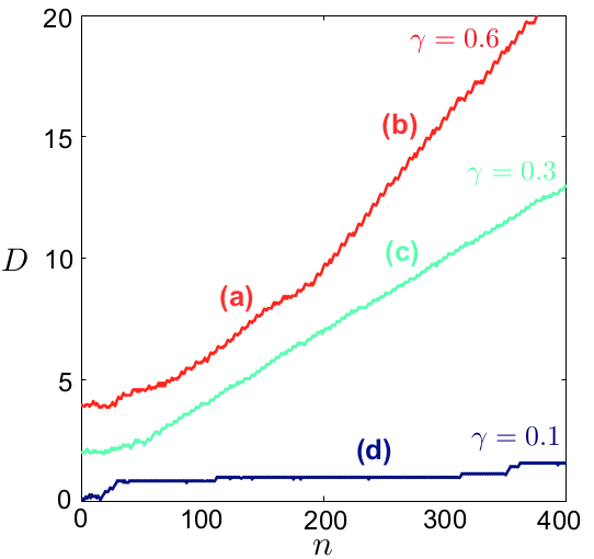
To show the effectivenesss of the reinforcement learning on swimmers, the four linked swimmer model is also tested. The figure below shows the propulsion policies learnt by the swimmer for different values of \(\gamma\), which means that the learning parameters \(\alpha\) and \(\gamma\) must be chosen carefully.
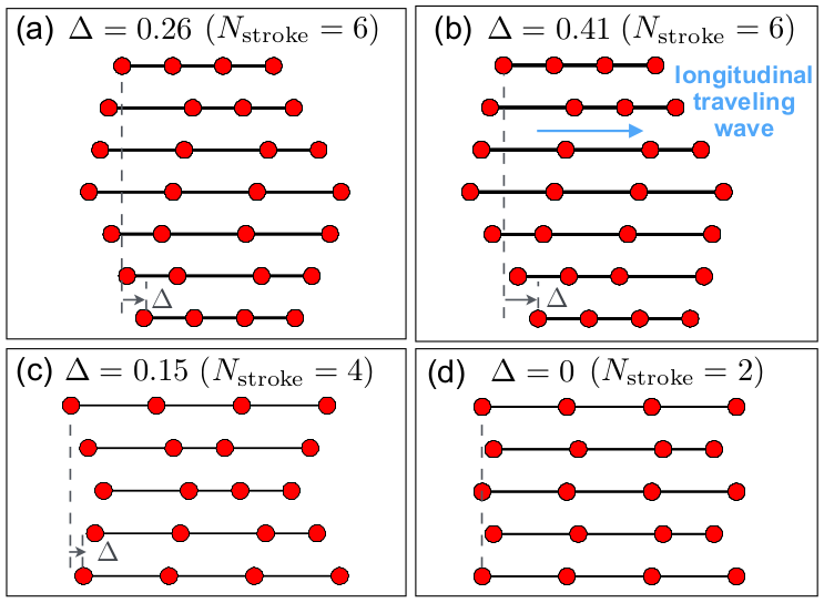
This figure shows that the swimmer can self-improve and evolve a better policy during the learning process.
At the initial stage, with \(\gamma=0.6\) the swimmer learns one propulsion policy (a). But after some steps of learning, the swimmer identifies a better propulsion policy (b) which is optimal for this model.
For \(\gamma=0.3\), The swimmer learns a different suboptimal propulsion policy (c) that can not be improved over the learning processs.
Th last test is for \(\gamma = 0.1\), where the swwimmer did not learn to swim (see also the figure below).
The following figure shows the influence of reinforcement learning parameter \(\gamma\) in the swimmer self-learning :
3. Article 3 : Modeling and finite element simulation of multi-sphere swimmers
In this article BCGP2020, the authors presented a finite element method to simulate micro-swimmers composed of multiple rigid bodies moving relatively to each other. A general model is studied numerically and the simple linked three spheres swimmer is tested. The general model is composed of \(n\) rigid bodies \(B_i\) linked all to a reference body \(B_n\). For simplicity reasons, all the bodies \(B_i\) are spheres.
Let \(\mathcal{F}_t\) be the domain occupied by the fluid at time \(t\). It is clear that \(\mathcal{F}_t= \mathbb{R}^3 \backslash\bigcup B_i\).
The equation describing the motion of \(n\) independent bodies is :
\[ \begin{cases} -\mu\Delta u + \nabla p = f,\qquad\qquad\qquad\qquad \text{in}\;\mathcal{F}_t,\\ \nabla .u = 0,\qquad\qquad\qquad\qquad\qquad\;\;\;\;\; \text{in}\;\mathcal{F}_t,\\ u = \mathbf{U}_i+\mathit{\omega}_i \times(x-x_i^{CM}(t))\qquad\;\;\;\;\;\text{on}\;\partial B_i,\\ m_i\dot{\mathbf{U}}_i = -F_{fluid},\qquad\qquad\qquad\qquad\; i = 1\cdots n,\\ J_i\dot{\mathit{\omega}}_i = -M_{fluid},\qquad\qquad\qquad\qquad\;\; i = 1\cdots n, \end{cases} \]
where :
-
\(u\) : the fluid velocity
-
\(p\) : the fluid pressure
-
\(\mathbf{U}\) : translational speed
-
\(\omega\) : angular speed
-
\(x^{CM}\) : the swimmer’s center of mass
-
\(m\) and \(J\) are the swimmer’s volume and geometric inertia tensors.
The variational formulation adressed to this equation is given by:
\[2\mu\int_{\mathcal{F}_t}D(u):D(\tilde{u})dx - \int_{\mathcal{F}_t}p\nabla .\tilde{u} dx + \sum_{i=1}^n m_i\mathbf{U}_i.\tilde{\mathbf{U}}_i + J_i\mathit{\omega}_i . \tilde{\mathit{\omega}_i} = \int_{\mathcal{F}_t}f.\tilde{u}dx \]
\[ \int_{\mathcal{F}_t}\tilde{p}\nabla.udx=0 \]
where \((\tilde{u}, \tilde{p},\tilde{\mathbf{U}},\tilde{\mathit{\omega}})\) are the test functions and \(\;\displaystyle{D(u) = \frac{1}{2}(\nabla u + \nabla u^T).}\)
Problem descretisation ???
The previous model is tested with same swimming gait mentionned in the article 1. We can see that the results found validate the ones in the first article, the center sphere is displaced \(0.16R\) in the positive direction at the end of the four stages.
The simulations of this work were obtained using the library FEEL++ toolboxe.
References on Swimming
-
[Najafi_2004] Ali Najafi, Ramin Golestanian. Simple swimmer at low Reynolds number: Three linked spheres. 2004. American Physical Society. doi.org/10.1103/PhysRevE.69.062901 linkDownload PDF
-
[nature] Jikeli, J., Alvarez, L., Friedrich, B. et al. Sperm navigation along helical paths in 3D chemoattractant landscapes. Nat Commun 6, 7985 (2015). doi.org/10.1038/ncomms8985 Download PDF
-
[bgp_cemracs_2019] Luca Berti, Laetitia Giraldi, Christophe Prud’Homme. Swimming at Low Reynolds Number. ESAIM: Proceedings and Surveys, EDP Sciences, 2019, pp.1 - 10, doi.org/10.1051/proc/202067004 Download PDF
-
[bcgp_three_spheres_2020] Luca Berti, Vincent Chabannes, Laetitia Giraldi, Christophe Prud’Homme. Modeling and finite element simulation of multi-sphere swimmers. 2020. hal-mines-paristech.archives-ouvertes.fr/ENSMP_CEMEF/hal-03023318v1 Download PDF
-
[gbcc_epje_2017] K. Gustavsson, L. Biferale, A. Celani, S. Colabrese Finding Efficient Swimming Strategies in a Three Dimensional Chaotic Flow by Reinforcement Learning Published on Eur. Phys. J. E (December 14, 2017) 10.1140/epje/i2017-11602-9 Download PDF
-
[purcell_1977] E.M. Purcell. Life at Low Reynolds Number, American Journal of Physics vol 45, p. 3-11 (1977). doi.org/10.1119/1.10903 Download PDF
References on Learning Methods
-
[gbcc_epje_2017] K. Gustavsson, L. Biferale, A. Celani, S. Colabrese Finding Efficient Swimming Strategies in a Three Dimensional Chaotic Flow by Reinforcement Learning Published on Eur. Phys. J. E (December 14, 2017) 10.1140/epje/i2017-11602-9 Download PDF
-
[Q-learning] Tsang, A.C., Tong, P., Nallan, S., Pak, O.S. (2018). Self-learning how to swim at low Reynolds number. arXiv: Fluid Dynamics.Download PDF