Simulations with articulated bodies

The geometry of this type of swimmers can be seen in the following picture :

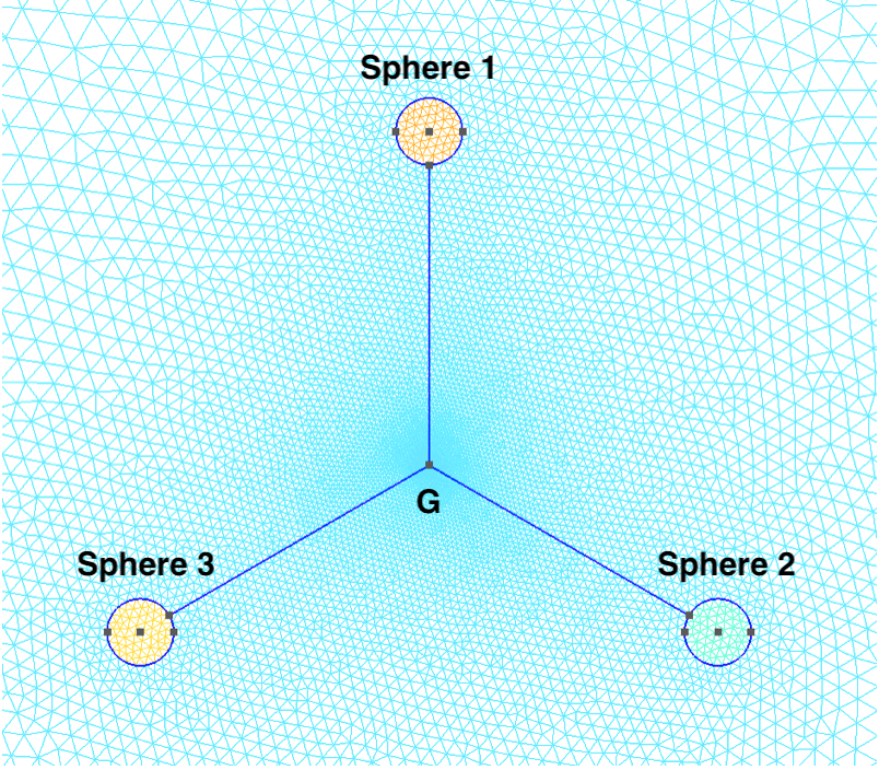
The three spheres are separated by an angle of \(120\) degrees. The swimmer is placed in a box filled with a fluid at low Reynolds number. In the figure, the \(G\) represents its center of mass.

The range of parameters is defined by :

The swimmer is placed in a rectangular box. The domain is thus defined by:

First application

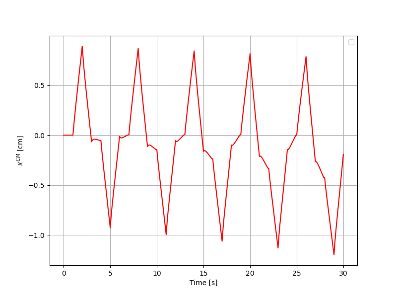
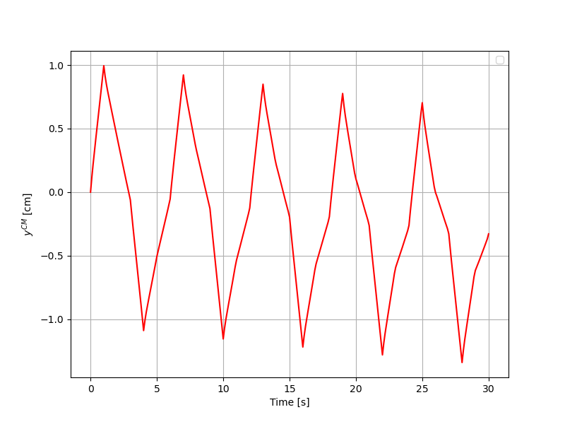
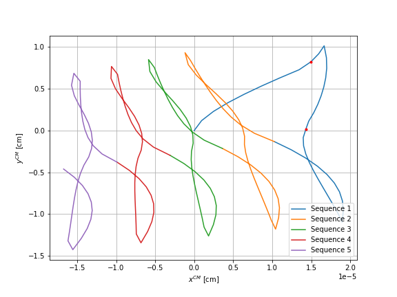
The first simulation is performed on 30 seconds. Every 6 seconds, the swimmer repeats the same sequence of movements. First, he contracts the upper sphere, the sphere \(1\), then the right sphere, sphere \(2\), and finally the left one, sphere \(3\). Afterwards, he extends his spheres in the same order. We represent the time evolution of the horizontal and vertical position of the center of mass of the swimmer. For these graphs we do not have verified results to make comparisons. The representations are given by :

Second application

To verify that the swimmer is moving in theoretical direction, we consider a sequence of four movements. First he contracts one sphere and then simultaneously the other two before extending the first sphere and finally simultaneously the other two. When we consider that the sphere \(1\), thus the upper sphere, moves alone, then the four movements are defined by :

Each movement takes one second. This sequence of movements should result that the swimmer’s center of mass moves downward without having a horizontal displacement.

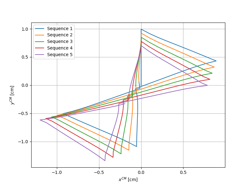
The first graph shows the displacement of the center of mass during \(8\) sequences of these four movements. The second graph shows only the displacement after each sequence. The orange line corresponds to the theoretical displacement.

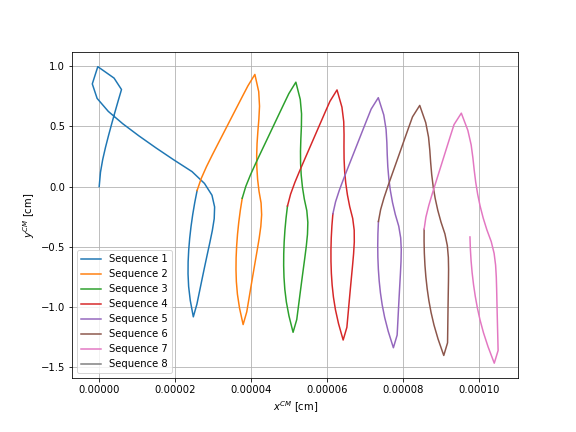
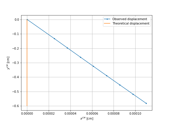
We simulate these \(8\) sequences of movement also in the case where the sphere \(2\) thus the right sphere moves alone and in the case where the sphere \(3\) moves alone.

We can notice that the order of error is more important for the cases of sphere \(2\) and the sphere \(3\) than for the case of sphere \(1\). By visualizing the displacements with Paraview, one can observe that this can be the result of the boundary effects of the rectangular domain. Thus, we have done the same simulations considering a large circular domain.

In this case the domain is defined by:

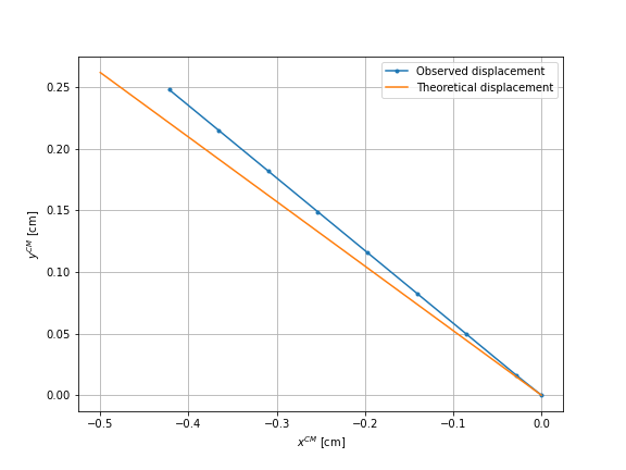
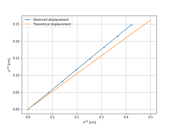
First application

We plot, for each case, the displacement during five sequences on the first graphs and the motion after each sequence on the second graph. The orange line represents the theoretical displacement. For the case of the sphere \(2\) and \(3\), we rotate the results so that it corresponds to the theoretical displacement of the case of the sphere \(1\), thus a vertical displacement only.

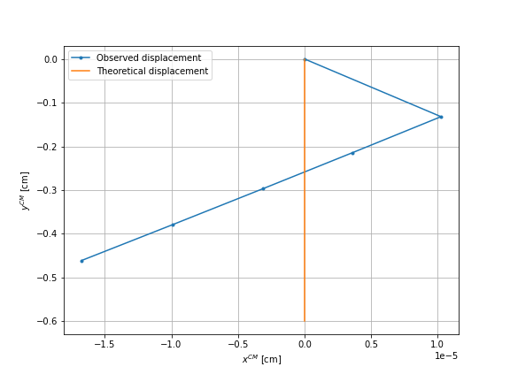
It can be observed that for all three cases a negligible horizontal displacement is obtained, an error of order \(10^{-5}\). However, the right graphs show that the first sequence of the four movements result in a different displacement than the following sequences. As this should not be the case, we will perform different checks to understand the reason for this difference.

Second application

First, we check that the displacement of the swimmer’s center of mass after each sequence is equal to the displacement of each sphere. We use the case of sphere \(1\). The four graphs visualize this motion, the orange line corresponds to the theoretical displacement.

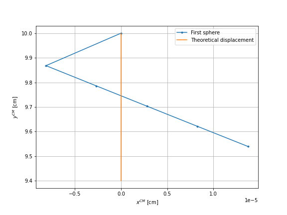
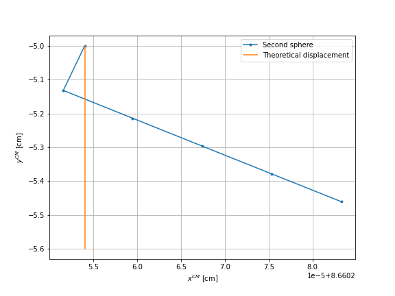
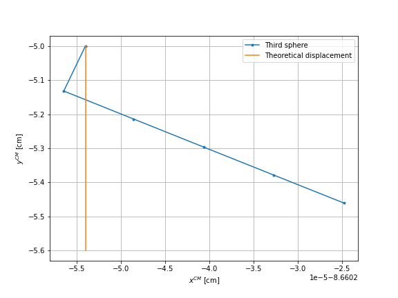
We can observe that the movements are similar. The error is more important for the spheres \(2\) and \(3\) than for the sphere \(1\) and the center of mass of the swimmer. The same observations are made for the other two cases.

Third application

Second, we display the number and the instants of remeshing for each case. The red points on the graphs, figures \(9\), \(11\), \(13\), correspond to these remeshes.

It can be seen that after the last remeshing, the displacement of the sequences remains the same. To make sure that the problem of the different displacement is caused by the initial mesh, we redo the same simulations using as initial mesh the one obtained after two sequences of four movements. The displacements are supposed to be identical to those of the third sequence.

We could not perform this check. The tool to reuse a mesh doesn’t exist yet in the python layer of Feel++.

Fourth application

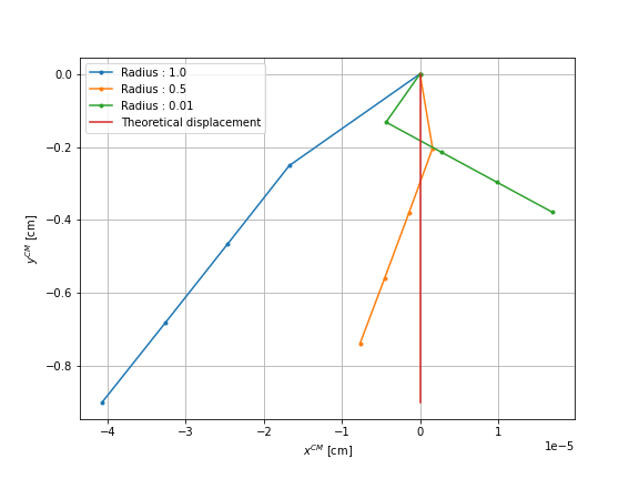
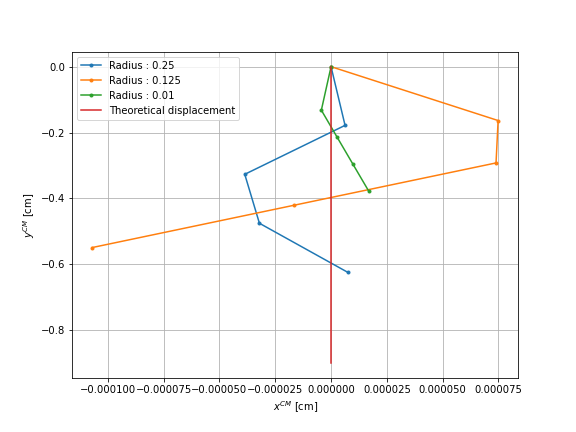
Third, we analyze the influence of the radius of the center sphere that builds the swimmer’s center of mass. Initially, its radius is equal to \(r = 0.01\). We consider the radii :

while keeping the mesh step fixed equal to \(0.2\). We show the displacement after each sequence of four movements in the case of sphere \(1\), comparing it to the one where the sphere of the center has the initial radius and to the theoretical displacement.

The table shows the number and instants of remeshing:

The different radii result in an error, hence a horizontal displacement, larger than the initial radius. The number of remeshes is also equal or greater than that of the reference case. Only for \(r = 0.5\) better results are obtained. For this reason, we consider the results for the same simulation using a radius equal to \(r = 0.5\) and a smaller mesh size for the spheres, equal to \(h = 0.1\) instead of \(h = 0.2\). The graph shows this comparison:

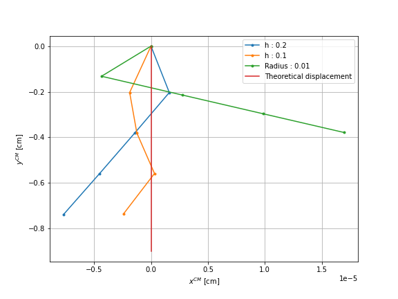
The error obtained for this mesh size is even smaller. However, this simulation requires \(53\) remeshes, the displacement is not periodic.