Boustrophedon decomposition path planning with obstacles

Table of Contents

1. Introduction
2. Boustrophedon decomposition algorithm
- 2.1. Description
- 2.2. Boustrophedon motion with obstacles
3. Implementation
4. Results
5. Conclusion

1. Introduction

Path planning is one of the most fundamental challenges in autonomous robotics. A robot must be able to move efficiently and safely in a complex environment, avoiding obstacles while reaching its destination optimally. In this context, the Boustrophedon decomposition algorithm is proving to be an effective approach to solving this problem. We will use the Boustrophedon motion algorithm to get the robot’s motion in a rectangular domain with obstacles.

2. Boustrophedon decomposition algorithm

2.1. Description

To detect the obstacles, we apply a ray tracing method. First, we use the pyvista library to create a surface from the mesh representing the environment with obstacles. Then we perform the ray tracing method to get the position of the obstacles. The method traces rays along the entire width of the domain and allows computing the points of intersection between each ray and the mesh. The number of points gives information about the presence of obstacles, which are stored in a graph.

To construct the graph, proceed as follows:

Initialize a list L = [[ x1min, y1min, y1max ]] initially containing the coordinates of the first open node.
We start by defining two starting points at the top and bottom of the environment.
Then, for each possible horizontal position (defined by i), ray tracing is performed along the width to find the points of intersection along this horizontal line. These intersection points delimit the open gaps between the obstacles.
If the number of intersection points increases relative to the previous position, an obstacle has been encountered.
So if the intersection points lie between y_min and y_max, we create a node whose coordinates will be removed from the L list and then add it to the graph.
On the other hand, if the number of intersection points decreases and the y_min and y_max are compressed between the intersection points.
We create a node whose coordinates will be removed from the list.
Update the list with the new coordinates and add the node to the graph.
Update previous_points with the intersection points obtained in this iteration.
Browse the nodes in the L list and add the missing nodes to the graph, checking if they’re already there.

To add edges to the graph:

All nodes in the graph are traversed.
For each node, we obtain the coordinates xmax and xmin, which represent the upper bound of the interval and the lower bound of the interval respectively.
If the absolute difference between xmax and xmin is very close to zero, this means that these two nodes share the same point on the x axis. In this case, add an edge between these two nodes in the graph to capture the relationship.

Next, traverse all the nodes in the graph and save the robot trajectories associated with each node in CSV files. We paste the CSV of the nodes to create the total CSV that the robot must follow to traverse the domain.

We then perform a depth-first search (DFS) on the edges of the graph to generate the robot’s complete movement paths. Each edge connects two adjacent nodes and represents a path between horizontal segments.

Finally, we use the python visualization library ( NetworkX) to show the graph, and we use our Boustrophedon algorithm to visualize the robot’s trajectory.

2.2. Boustrophedon motion with obstacles

Inputs:

height and width: The height and width of the computational domain.
delta_x: The horizontal step size to divide the environment into cells.
delta_y: The vertical step size.

Ray tracing:

Trace the rays on the mesh to detect intersections with obstacles.

Constructing the graph:

Given: L = [x1min, y1min, y1max].

Check if intersection points has increasing:
- loop on list
  - Check whether (X[i, i, even] = Y_new_min) is in [y_min ,y_max].
    
    If yes
    
    1) Create node N[X_j_min,y_j_min, X, y_j_max].
    
    2°) Delete [X_j_min, y_j_min, y_j_max] from the list.
    
    3°) Add [X, y_i_plus_1_min, y_j_max] to the list.
    
    4°) Add [X, y_j_min, y_new_max] to the list.
Check if intersection points has decreasing:
- loop on list
  - Check if (y_i_minus_1 < y_j_max < y_i) or (y_i_minus_1 < y_j_min < y_i).
    
    If yes
    
    1°) Create node N[X_j_min,y_j_min, X, y_j_max].
    
    2°) Delete [X_j_min,y_j_min, y_j_max] from the list.
    
    3°) Add [X, y_i_minus_1, y_i] to the list (if not already present).
At the end, the last cell is added to the graph.
Finally, edges are added to the graph G to connect adjacent cells with the same x_min and x_max limits.
We construct the CSV of each node and then connect them to obtain the total CSV, which gives us the robot’s path.

3. Implementation

We have implemented the Boustrophedon decomposition algorithm in python.

from boustrophedon_motion import Boustrophedon_Motion as BM
from os import mkdir, chdir, path
import matplotlib.pyplot as plt
import networkx as nx
import pyvista as pv
import csv

class Boustrophedon_Decomposition_2D:

    """
    This class implements the Boustrophedon Decomposition Path Planning Algorithm
    for a 2D environment with obstacles.

    """

    def __init__(self, height, width, delta_x, delta_y):
        self.x1min = 0
        self.y1min = 0
        self.x1max = 0
        self.y1max = height
        self.height = height
        self.width = width
        self.delta_x = delta_x
        self.delta_y = delta_y
        self.xmin_previous = self.x1min
        self.ymin_previous = self.y1min
        self.G = nx.Graph()


    def ray_trace(self, start, stop):
        mesh = pv.read("path_with_obstacle.msh") # read the mesh
        surf = pv.PolyData(mesh.points, mesh.cells) # create a surface from the mesh
        points, ind = surf.ray_trace(start, stop) # ray trace from start to stop

        return points, ind


    def build_graph(self):

        previous_points = ([self.x1min, self.y1min], [self.x1max, self.y1max])
        L = [[self.x1min, self.y1min, self.y1max]] # list of open nodes
        i = 0

        while i < self.width:
            i += self.delta_x
            start = [i, -1, 0]
            stop = [i, 4, 0]
            points, ind = self.ray_trace(start, stop)

            to_remove = [] # list of nodes to remove from the list

            if len(points) > len(previous_points):
                y = points[:, 1] # vector of y coordinates of intersection points

                for vec in L:
                    y_j_min = vec[1] # y coordinate of the lower bound of the interval
                    y_j_max = vec[2] # y coordinate of the upper bound of the interval

                    j=0
                    for j in range(len(y)//2):

                        if y_j_min < y[2*j + 1] < y_j_max:
                            # Create new node in the graph
                            x_j_min = vec[0]
                            N = ((x_j_min, y_j_min, i, y_j_max))

                            L.remove([x_j_min, y_j_min, y_j_max])

                            y_i_plus_1_min = y[2*j+2]
                            L.append([i, y_i_plus_1_min, y_j_max])

                            y_new_max = y[2*j+1]
                            L.append([i, y_j_min, y_new_max])

                            self.G.add_node(N)

            if len(points) < len(previous_points):
                y = points[:, 1] #vector of y coordinates of intersection points

                for vec in L:
                    y_j_min = vec[1] # y coordinate of the lower bound of the interval
                    y_j_max = vec[2] # y coordinate of the upper bound of the interval

                    j=0
                    for j in range(len(y)//2):

                        if (y[2*j] < y_j_max < y[2*j+1]) or (y[2*j] < y_j_min < y[2*j+1]):
                            # Create new node in the graph
                            x_j_min = vec[0] #x coordinate of the lower bound of the interval
                            N = ((x_j_min, y_j_min, i, y_j_max)) # new node
                            to_remove.append([x_j_min, y_j_min, y_j_max]) #remove this node from the list

                            L.append([i, y[2*j], y[2*j+1]]) #add the new node to the list

                            self.G.add_node(N) # add the new node to the graph

            for item in to_remove:

                if item in L:
                    L.remove(item) # remove the node from the list

            previous_points = points # update the previous points

        # Add last open nodes to the graph
        for vec in L:
            x_j_min = vec[0] # x coordinate of the lower bound of the interval
            y_j_min = vec[1] # y coordinate of the lower bound of the interval
            y_j_max = vec[2] # y coordinate of the upper bound of the interval
            N = ((x_j_min, y_j_min, self.width, y_j_max))

            if N not in self.G.nodes:
                self.G.add_node(N)

        # Add edges to the graph
        for n in nx.nodes(self.G):
            xmax = n[2] # x coordinate of the upper bound of the interval

            for m in nx.nodes(self.G):
                xmin = m[0] # x coordinate of the lower bound of the interval

                if abs(xmax - xmin) < 1e-10:
                    self.G.add_edge(n, m, value=1) # add edge between n and m



    def save_node_path_as_csv(self, node, radius, delta, step_H, step_V, time, dt,i):
        height =  node[3] - node[1] # height of the node
        width = node[2] - node[0] # width of the node

        folder_name = "node" + str(i) # name of the folder
        if not path.exists(folder_name): # if the folder doesn't exist
            mkdir(folder_name) # create the folder
        chdir(folder_name) # go to the folder

        # print("height =", height)
        # print("width =", width)
        BM.generate_file_csv(height, width, radius, node[0], node[1], delta, step_H, step_V, time, dt)

        chdir("..") # go back to the previous folder


    def save_node_paths_as_csv(self,radius, delta, step_H, step_V, time, dt):
        i = 0

        for node in self.G.nodes:
            self.save_node_path_as_csv(node,radius, delta, step_H, step_V, time, dt, i)
            i += 1


    def traverse_graph_dfs_edges(self, dt):
        ordered_edges = list(nx.dfs_edges(self.G)) # list of edges in the order of the DFS
        list_node = list(self.G.nodes) # list of nodes in the graph

        with open("boustrophedon_path.csv", mode='w', newline='') as boustrophedon_file:
            writer_bf = csv.writer(boustrophedon_file, delimiter=',')
            total_time = 0
            initial_node = ordered_edges[0][0] # initial node of the path
            i = list_node.index(initial_node) # index of the initial node

            with open((f"node{i}/position.csv"), newline='') as csvfile:
                last_element = csvfile.readlines()[-1] # last element of the file
                csvfile.seek(0) # go back to the beginning of the file
                read = csvfile.read() # read the file
                boustrophedon_file.write(read) # write the file in the boustrophedon file
                total_time = float(last_element.split(",")[2]) # total time of the path

            for edge in ordered_edges:
                node0 = edge[0]
                node1 = edge[1]

                i = list_node.index(node0) # index of the first node
                j = list_node.index(node1) # index of the second node

                with open((f"node{i}/position.csv"), newline='') as csvfile:
                    reader = csv.reader(csvfile, delimiter=',') #read csv file
                    next(reader) #skip the first line

                    last_element = csvfile.readlines()[-1] # last element of the file
                    last_cell_y = float(last_element.split(",")[1])
                    last_cell_x = float(last_element.split(",")[0])
                    last_time = total_time

                    # print(f"last_element_node{i} =", last_element)
                    # print(f"last_cell_x_node{i} =", last_cell_x)
                    # print(f"last_cell_y_node{i} =", last_cell_y)
                    # print()
                    # print("-----------------------------------")

                with open((f"node{j}/position.csv"), newline='') as csvfile2:
                    reader = csv.reader(csvfile2, delimiter=',') #read csv file
                    next(reader) #skip the first line

                    first_element = csvfile2.readlines()[0] # first element of the file
                    first_cell_y = float(first_element.split(",")[1]) # y coordinate of the first cell
                    first_cell_x = float(first_element.split(",")[0]) # x coordinate of the first cell

                    # print(f"first_element_node{i} =", first_element)
                    # print(f"first_cell_x_node{i} =", first_cell_x)
                    # print(f"first_cell_y_node{i} =", first_cell_y)
                    # print()
                    # print("-----------------------------------")

                cells = [] # list of cells of the edge
                y = last_cell_y # y coordinate of the cell

                if last_cell_y > first_cell_y: # if the last cell is above the first cell


                    while abs(y - first_cell_y)>1e-10:
                        x = last_cell_x

                        while x < first_cell_x:
                            x += self.delta_x
                            last_time += dt
                        cells.append([x, last_cell_y, last_time]) # add the cell to the list


                        y -= self.delta_y
                        last_time += dt
                        cells.append([x, y, last_time]) # add the cell to the list
                else:

                    while abs(y - first_cell_y)>1e-10:
                        x = last_cell_x
                        y += self.delta_y
                        last_time += dt
                        cells.append([x, y, last_time])

                if last_cell_x < first_cell_x:
                    x = last_cell_x

                    while abs(x - first_cell_x)>1e-10:
                        x += self.delta_x
                        last_time += dt
                        cells.append([x, y, last_time])

                else:
                    x = last_cell_x

                    while abs(x - first_cell_x)>1e-10:
                        x -= self.delta_x
                        last_time += dt
                        cells.append([x, y, last_time])

                # save the path of the edge in a CSV file
                file_name = f"path_edge_{i}_{j}.csv"

                with open(file_name, mode='w', newline='') as file:
                    writer = csv.writer(file, delimiter=',')
                    writer.writerow(['x', 'y', 'time'])  # the headers

                    for point in cells:
                        writer.writerow(point) # write the cells in the file
                        writer_bf.writerow(point) # write the cells in the boustrophedon file

                total_time = last_time

                with open((f"node{j}/position.csv"), newline='') as csvfile2:
                    reader = csv.reader(csvfile2, delimiter=',') #read csv file
                    next(reader) #skip the first line
                    # next(reader) #skip the second line

                    for row in reader:
                        total_time += dt # add dt to the time
                        row[2] = total_time # update the time
                        writer_bf.writerow(row) # write the cells in the boustrophedon file



    def draw_graph(self):
        # some math labels
        labels = {} # labels for nodes

        for i in range(len(self.G.nodes)):
            labels[list(self.G.nodes)[i]] = i + 1 # label nodes from 1 to n

        # draw graph with labels in math mode
        pos = {} # positions for all nodes

        for l in nx.nodes(self.G):
            xmin = l[0]
            xmax = l[2]
            ymin = l[1]
            ymax = l[3]
            pos[l] = [(xmin + xmax) / 2, (ymin + ymax) / 2] # position of the node

        legend = {v: k for k, v in labels.items()}
        print("{:<20} {:<20} {:<20} {:<20} {:<20}".format('Node', 'xmin', 'ymin',
                                                          'xmax', 'ymax'))

        # print each data item.
        for key, value in legend.items():
            coord = value
            print("{:<20} {:<20} {:<20} {:<20} {:<20}".format(key, coord[0], coord[1],
                                                              coord[2], coord[3]))

        nx.draw_networkx(self.G, labels=labels, with_labels=True, font_weight='bold',
                         pos=pos)

        plt.show()

4. Results

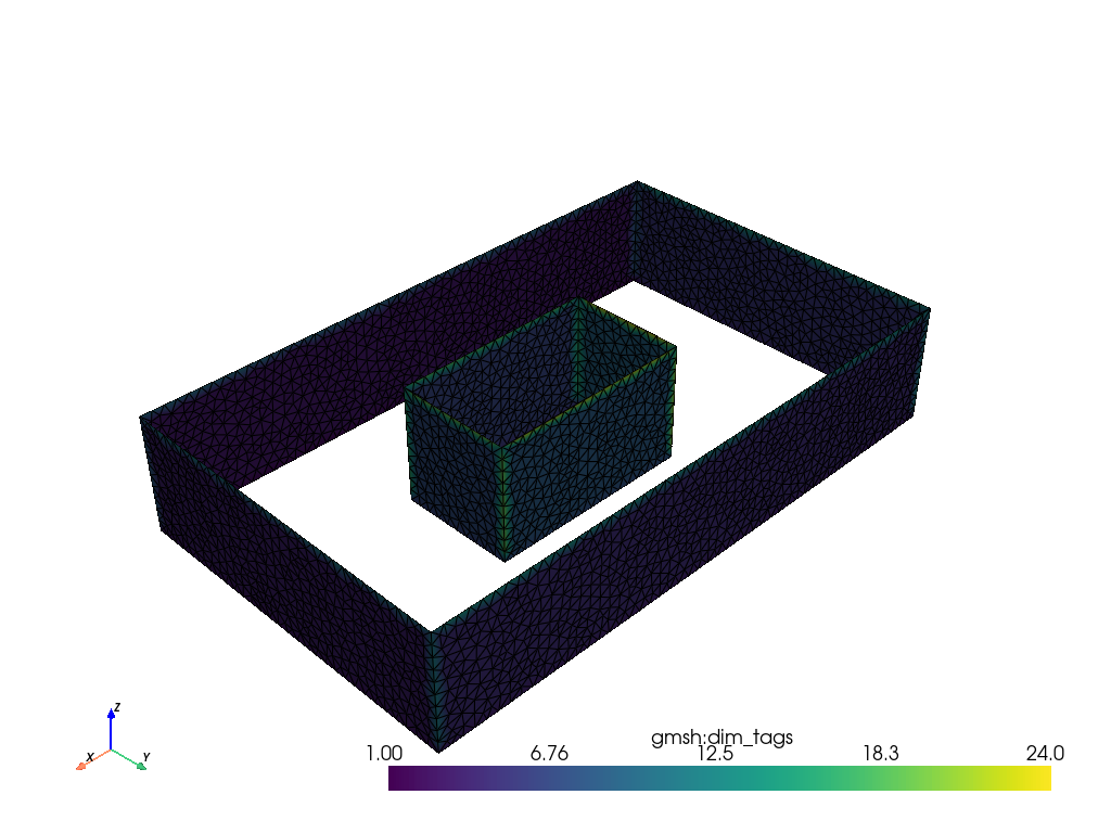
We read the mesh with the Pyvista library and display the mesh.

In the case of a single obstacle, we have the following figure.

import numpy as np
import matplotlib.pyplot as plt
import csv

# print(mesh.cells_dict)
mesh.cells
# read mesh.cells with pyvista
import pyvista as pv
mesh = pv.read("path_with_obstacle.msh")
mesh.plot(show_edges=True, line_width=1)

Results

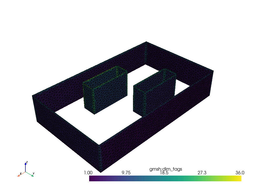
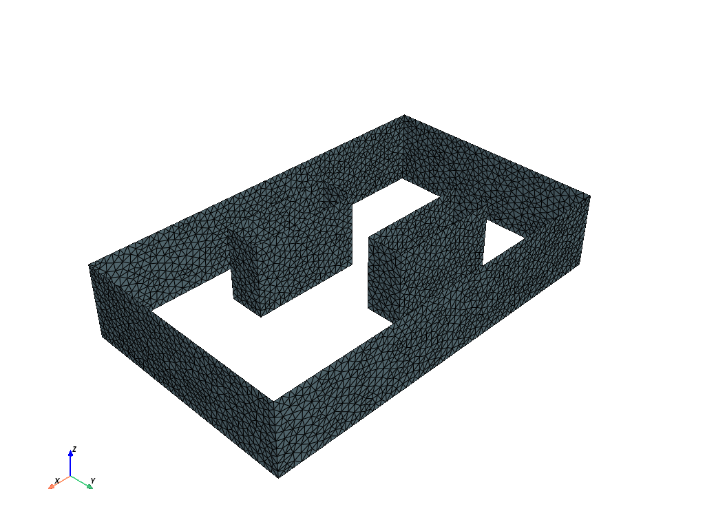
And here we display the domain mesh and the two obstacles with meshio.

import numpy as np
import matplotlib.pyplot as plt
import csv

# print(mesh.cells_dict)
mesh.cells
# read mesh.cells with pyvista
import pyvista as pv
mesh = pv.read("path_with_obstacles.msh")
mesh.plot(show_edges=True, line_width=1)

Results

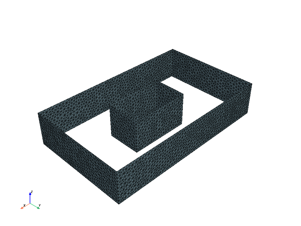
The Pyvista library and Polydata (pv.PolyData) are used to display the mesh surface, i.e. the surface of the domain and obstacles.

In the first case, we have a single obstacle.

import pyvista as pv

mesh = pv.read("path_with_obstacle.msh")
surf = pv.PolyData(mesh.points, mesh.cells)
surf.plot(show_edges=True, line_width=1)

Results

In the second case, we have two obstacles.

import pyvista as pv

mesh = pv.read("path_with_obstacles.msh")
surf = pv.PolyData(mesh.points, mesh.cells)
surf.plot(show_edges=True, line_width=1)

Results

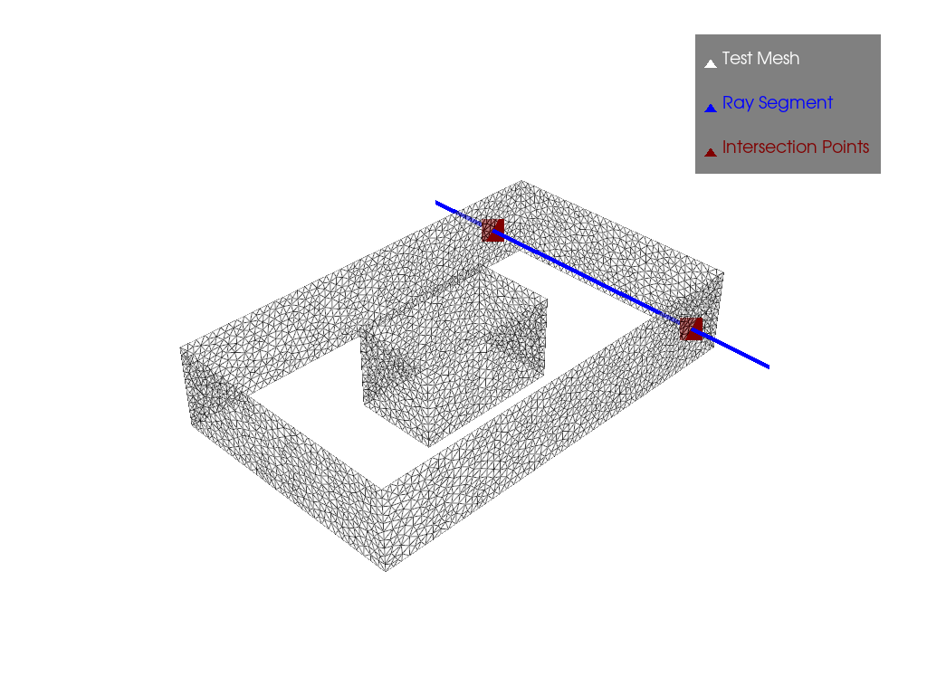
It’s on these surfaces that we did our ray tracing with ray_tracing to be able to form the graph with the connectivity changes. And we have the results in the case where there is only one obstacle:

Here we have our plot with two points of intersection between the ray and the surface.

# Define line segment
start = [0.5, -1, 0.5]
stop = [0.5, 4, 0.5]

# Perform ray trace
points, ind = surf.ray_trace(start, stop)

# Create geometry to represent ray trace
ray = pv.Line(start, stop)
intersection = pv.PolyData(points)


# Render the result
p = pv.Plotter(off_screen=True)
p.add_mesh(surf, show_edges=True, opacity=0.5, color="w", lighting=False, label="Test Mesh")
p.add_mesh(ray, color="blue", line_width=5, label="Ray Segment")
p.add_mesh(intersection, color="maroon", point_size=25, label="Intersection Points")
p.add_legend()
p.show()

Results

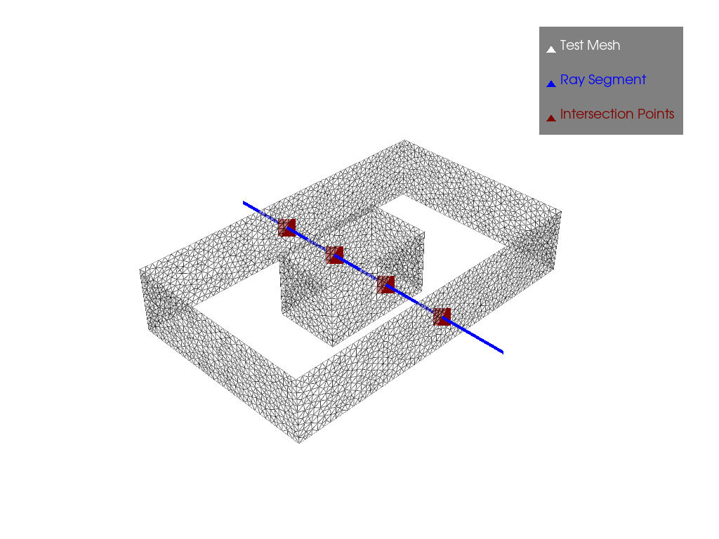
In the case where the obstacle is encountered while traversing the domain, we see a change in connectivity, i.e. the number of points increases from 2 to 4. And if the ray no longer touches the obstacle, there’s also a change in connectivity, but in this case the number of points drops from 4 to 2, and that’s how we’ve formed our graph.

# Define line segment
start = [0.5, -1, 0.5]
stop = [0.5, 4, 0.5]

# Perform ray trace
points, ind = surf.ray_trace(start, stop)

# Create geometry to represent ray trace
ray = pv.Line(start, stop)
intersection = pv.PolyData(points)


# Render the result
p = pv.Plotter(off_screen=True)
p.add_mesh(surf, show_edges=True, opacity=0.5, color="w", lighting=False, label="Test Mesh")
p.add_mesh(ray, color="blue", line_width=5, label="Ray Segment")
p.add_mesh(intersection, color="maroon", point_size=25, label="Intersection Points")
p.add_legend()
p.show()

Results

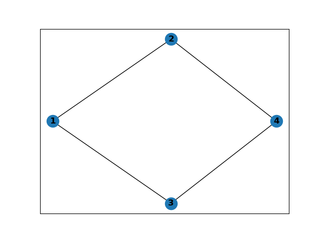
We have the following graphs:

Nodes are represented by the numbers (1, 2, 3 and 4) whose positions are represented by [(xmin + xmax) / 2, (ymin + ymax) / 2] and edges are added to the G graph to connect adjacent cells with the same x_min and x_max limits. In this way, we have an adjacent graph that allows the robot to cover the working domain without touching the obstacle.

For a single obstacle in the domain, we have the following graph:

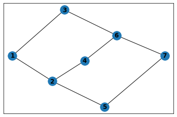
And for two obstacles we have the following figure :

Once the graph has been obtained, we construct the csv of the nodes thus obtained. Then we glue them together to obtain the total csv of the workspace, which gives us the robot’s trajectory.

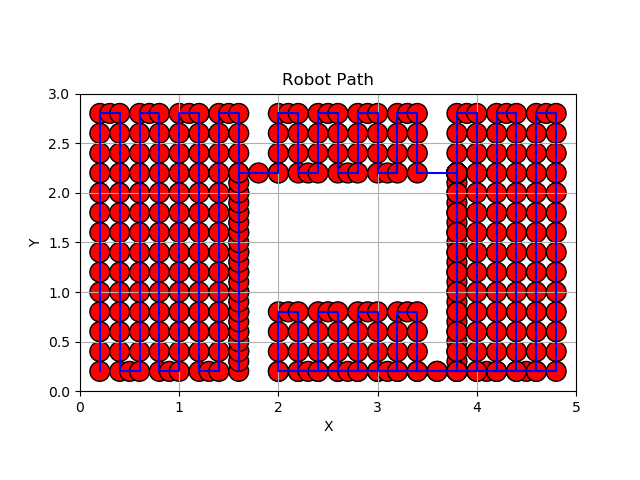
In the case of a single obstacle, after creating the four nodes, we see that the path is as follows:

The robot traverses the area of node1, then enters the area of node2 via the edge linking the two nodes. It then continues its sweep in the area of node4, ending up in the area of node3. The following figure shows the robot’s path through the working area without touching the obstacle.

5. Conclusion

In this chapter, we implemented the Boustrophedon decomposition algorithm to generate the robot trajectory in a rectangular area with obstacles. We used the ray tracing method to detect the obstacles and to obtain the graph. Finally, we were able to show the robot’s trajectory.