 .pdf
.pdf
Stationary Stokes equations
1. Mathematical formulation
Let \(\Omega \subseteq \mathbb{R}^d\), \(d = 2\) or \(d=3\), be the domain of the fluid and \(\partial \Omega\) its boundary. The boundary satisfies \(\partial \Omega = \Gamma_D \cup \Gamma_N\), where \(\Gamma_D\) denotes the portion of the boundary where the Dirichlet boundary conditions are imposed, and \(\Gamma_N\) the portion where Neumann boundary conditions are imposed. We note \(u : \Omega \mapsto \mathbb{R}^d\) and \(p : \Omega \mapsto \mathbb{R}\) respectively the velocity and the pressure of the fluid. Let \(\mu \in \mathbb{R}^{+}\) be its dynamic viscosity. The stationary Stokes equations link these variables by the following system:
where \(f : \Omega \mapsto \mathbb{R}^d\) represents external forces and \(D(u) = \frac{1}{2}(\nabla u + \nabla u^{T})\) is the deformation tensor.
Variational formulation
We suppose \(f \in L^2(\Omega)^d\) and choose \(v \in H^1(\Omega)^d\), \(q \in L^2_0(\Omega) = \{ q \in L^2(\Omega) | \int_{\Omega} q = 0\}\) as the test functions. The variational formulation of \ref{p:1} is given by :
Find \((u,p) \in H^1(\Omega)^d \times L^2_0(\Omega)\) such that:
We denote:
where \(a\) is a bilinear form and \(b\) is a linear form. The variational formulation can be rewritten as:
Let \(X = H^1(\Omega)^d, M = L^2_0(\Omega)\). Find \((u,p) \in X \times M \) such that:
Using the Lax-Milgram theorem, one can prove that this variational formulation has a unique solution \((u,p)\). We approximate this solution by the Galerkin method using a \(\mathbb{P}_2/\mathbb{P}_1\) finite element discretization. We note \(X_h \subset X\) and \(M_h \subset M\) two Lagrangian finite element spaces of dimension \(N_u\) and \(N_p\).
We will detail two different methods to solve this variational problem. The differences between the two methods get obvious when implementing them. The first method requires the definition of a composite function space \(X_h \times M_h\) which results in more implicit integrals calculations, while in the second method the function spaces and integrals are defined one by one.
First resolution method
A first method is to solve directly the discrete variational problem:
Find \((u_h,p_h) \in X_h \times M_h\) such that:
Second resolution method
The second method consists in using the matrix formulation of the variational problem. Let \((\phi)_i\) be the basis of \(X_h\) and \((\varphi)_i\) the basis of \(M_h\). We have:
The discrete variational formulation is rewritten as :
Taking \(v_h = (\phi)_j\) and \(q_h = (\varphi)_j\), one find the matrix formulation:
where:
2. Implementation
We will detail the implementation of these two resolution methods for stationary Stokes equations.
A C++ file contains the implementation of the resolution of Stokes equations. For its execution we must define two other files, a geo file for the definition of the geometry and a cfg file, Stokes_config.cfg. The latter contains the configuration of the problem: the name of the geometry file and the definition of some function expressions.
The execution in \(2\)D and \(3\)D is respectively realized by the command line:
./feelpp_qs_stokesCeline_2d --config-file Cases/Stokes_config.cfg
./feelpp_qs_stokesCeline_3d --config-file Cases/Stokes_config.cfg
We will first show the different steps of the C++ file and then its configuration in the cfg file.
Mesh
We start by loading the mesh:
typedef Mesh<Simplex<FEELPP_DIM,1>> mesh_type; (1)
auto mesh = loadMesh(_mesh=new mesh_type); (2)| 1 | Definition of the mesh data structure, where d = FEEL_DIM, the dimension of the domain. |
| 2 | Loading the mesh from the geo file indicated in the cfg file. |
Function spaces
First resolution method
For the first resolution method, when considering directly the discrete variational formulation, we define a composite function space: \(\mathbb{P}_2/\mathbb{P}_1/\mathbb{P}_0\).
The definition of this composite function space is given by:
typedef Lagrange<2, Vectorial> basis_u_type; (1)
typedef Lagrange<1, Scalar> basis_p_type; (2)
typedef Lagrange<0, Scalar> basis_l_type; (3)
typedef bases<basis_u_type,basis_p_type,basis_l_type> basis_type; (4)
typedef FunctionSpace<mesh_type, basis_type> space_type; (5)
auto Xh = space_type::New(mesh); (6)| 1 | Definition of \(\mathbb{P}_2^d\) Lagrange finite element. |
| 2 | Definition of \(\mathbb{P}_1\) Lagrange finite element. |
| 3 | Definition of \(\mathbb{P}_0\) Lagrange finite element. |
| 4 | Collection of the basis functions of the composite function space. |
| 5 | Definition of the composite function space. |
| 6 | Initialization of a variable containing the type of the composite function space. |
We can thus define the different elements:
auto U = Xh->element(); (1)
auto u = U.element<0>();
auto p = U.element<1>();
auto lambda_1 = U.element<2>();
auto V = Xh->element(); (2)
auto v = V.element<0>();
auto q = V.element<1>();
auto lambda_2 = V.element<2>();| 1 | Definition of the trial elements, initialized to \(0\). |
| 2 | Definition of the test elements, initialized to \(0\). |
The \(\mathbb{P}_0\) Lagrangian elements \(\lambda_1\) and \(\lambda_2\) are used to impose the two conditions :
Second resolution method
While considering the matrix formulation one defines separately the three function spaces:
auto Xh = Pchv<2>(mesh); (1)
auto Mh = Pch<1>(mesh); (2)
auto P0ch = Pch<0>(mesh); (3)

auto u = Xh->elementPtr(); (4)
auto p = Mh->elementPtr();
auto lambda = P0ch->elementPtr();| 1 | Initialization space spanned by \(\mathbb{P}_2^d\) Lagrange finite element. |
| 2 | Initialization space spanned by \(\mathbb{P}_1\) Lagrange finite element. |
| 3 | Initialization space spanned by \(\mathbb{P}_0\) Lagrange finite element. |
| 4 | Definition of elements. |
The matrix formulation is given in the previous paragraph. We add the blocks \(C\) and \(C^T\):
where \(C = (c(\psi_i, \varphi_j))_{i,j} = (\int_{\Omega} \psi_i \varphi_j)_{i,j}\), and \((\psi)_i\) a basis of the \(\mathbb{P}_0\) Lagrangian finite element space.
We define the different blocks of this matrix and of the two vectors:
BlocksBaseGraphCSR myblockGraph(3,3); (1)
myblockGraph(0,0) = stencil(_test=Xh,_trial=Xh,_diag_is_nonzero=false,_close=false)->graph(); (2)
myblockGraph(0,1) = stencil(_test=Xh,_trial=Mh,_diag_is_nonzero=false,_close=false)->graph(); (3)
myblockGraph(1,0) = stencil(_test=Mh,_trial=Xh,_diag_is_nonzero=false,_close=false)->graph(); (4)
myblockGraph(1,2) = stencil(_test=Mh,_trial=P0ch,_diag_is_nonzero=false,_close=false)->graph(); (5)
myblockGraph(2,1) = stencil(_test=P0ch,_trial=Mh,_diag_is_nonzero=false,_close=false)->graph(); (6)
auto A = backend()->newBlockMatrix(_block=myblockGraph); (7)

BlocksBaseVector<double> myblockVec(3); (8)
myblockVec(0,0) = backend()->newVector(Xh);
myblockVec(1,0) = backend()->newVector(Mh);
myblockVec(2,0) = backend()->newVector(P0ch);
auto F = backend()->newBlockVector(_block=myblockVec,_copy_values=false); (9)

BlocksBaseVector<double> myblockVecSol(3); (10)
myblockVecSol(0,0) = u;
myblockVecSol(1,0) = p;
myblockVecSol(2,0) = lambda;
auto UVec = backend()->newBlockVector(_block=myblockVecSol, _copy_values=false);(11)| 1 | Definition of the block matrix. |
| 2 | Definition of \(A\) by indicating its position in the matrix and the space of the test and trial elements. |
| 3 | Defintion of \(B^T\). |
| 4 | Defintion of \(B\). |
| 5 | Defintion of \(C^T\). |
| 6 | Defintion of \(C\). |
| 7 | Initialization of this block matrix in variable A. |
| 8 | Definition of the right vector with specification of element spaces. |
| 9 | Initialization of this vector in variable F. |
| 10 | Definition of the left vector with specification of elements. |
| 11 | Initialization of this vector in variable UVec. |
Expressions We initialize the expressions defined in the cfg file:
auto f = expr<FEELPP_DIM,1>(soption("functions.f")); (1)
auto mu = expr(soption("functions.mu")); (2)
auto h = expr<FEELPP_DIM,1>(soption("functions.h")); (3)
auto p_exact = expr(soption("functions.p")); (4)
auto u_exact = expr<FEELPP_DIM,1>(soption("functions.u")); (5)| 1 | Expression f used for the external forces. |
| 2 | Expression mu used for the fluid viscosity. |
| 3 | Expression h used for the Dirichlet conditions. |
| 4 | Expression p_exact used for the exact solution for the pressure. |
| 5 | Expression u_exact used for the exact solution for the velocity. |
Integrals and resolution
We can then define the integrals.
First resolution method
For this first method, we define a bilinear form a and a linear form l, adding to them the respective integrals. The position of the blocks is managed implicitly by the composite function space. In the names of the mathematical functions used, for example grad and gradt, the t at the end indicates that it is applied to a trial element.
auto l = form1(_test = Xh); (1)
l = integrate(_range = elements(mesh),_expr = inner(f,id(v))); (2)

if (mesh->hasAnyMarker({"Neumann"})) (3)
    l += integrate(_range = markedfaces(mesh,"Neumann"),_expr = inner(expr<FEELPP_DIM,1>(soption("functions.g")),id(v)));

auto a = form2(_trial = Xh,_test = Xh); (4)
a = integrate(_range = elements(mesh),_expr = 2 * mu * inner(0.5*(gradt(u)+trans(gradt(u))),0.5*(grad(v)+trans(grad(v))))); (5)
a += integrate(_range = elements(mesh),_expr = -idt(p)*div(v)+id(q)*divt(u)); (6)
a += integrate( _range = elements(mesh),_expr = idt(lambda_1)*id(q)+id(lambda_2)*idt(p)); (7)

a += on( _range = markedfaces(mesh,"Dirichlet"), _rhs = l, _element = u, _expr = h); (8)| 1 | Definition of linear form l. |
| 2 | Add the integral \(F(v)\) to l. |
| 3 | Add the Neumann conditions \(G(v)\) to l, if defined. |
| 4 | Definition of bilinear form a. |
| 5 | Add the integral \(a(u,v)\) to a. |
| 6 | Add the integral \(-b(u,q)\) and \(b(v,p)\) to a. |
| 7 | Add the integral \(c(\lambda_1,q)\) and \(c(\lambda_2,p)\) to a. |
| 8 | Add the Dirichlet conditions to a. |
The resolution is then done by the command:
a.solve( _rhs=l, _solution = U);Second resolution method
For the second method each block of the matrix A and the vector F is defined separately. When defining the integrals it will be necessary to indicate manually the position of each block.
auto l = form1(_test=Xh,_vector=F,_rowstart=0); (1)
l += integrate(_range=elements(mesh),_expr = inner(f,id(u))); (2)

if ( mesh->hasAnyMarker({"Neumann"})) (3)
    l += integrate(_range = markedfaces(mesh,"Neumann"),_expr = inner(expr<FEELPP_DIM,1>(soption("functions.g")),id(u)));

auto a = form2(_trial=Xh,_test=Xh,_matrix=A, _rowstart=0,_colstart=0); (4)
a += integrate(_range = elements(mesh),_expr = 2*mu*inner(0.5*(gradt(u)+trans(gradt(u))),0.5*(grad(u)+trans(grad(u))))); (5)

form2(_trial=Mh,_test=Xh,_matrix=A,_rowstart=0,_colstart=1) += integrate(_range=elements(mesh),_expr= -idt(p)*div(u)); (6)
form2(_trial=Xh,_test=Mh,_matrix=A,_rowstart=1,_colstart=0) += integrate(_range=elements( mesh ),_expr= id(p)*divt(u)); (7)
form2(_trial=P0ch,_test=Mh,_matrix=A,_rowstart=1,_colstart=2) += integrate(_range=elements(mesh),_expr= idt(lambda)*id(p)); (8)
form2(_trial=Mh,_test=P0ch,_matrix=A,_rowstart=2,_colstart=1) += integrate(_range=elements(mesh),_expr= id(lambda)*idt(p)); (9)

a += on( _range = markedfaces(mesh,"Dirichlet"), _rhs = F, _element = *u, _expr = h); (10)

backend(_rebuild=true)->solve( _matrix=A, _rhs=F, _solution=UVec ); (11)| 1 | Definition of linear form l and its position in the vector F. |
| 2 | Add the block \(F\) to l. |
| 3 | Add the Neumann conditions \(G\) to l if defined. |
| 4 | Definition of bilinear form a and its position in the matrix A. |
| 5 | Add the block \(A\) to a. |
| 6 | Add the block \(B^T\). |
| 7 | Add the block \(B\). |
| 8 | Add the block \(C^T\). |
| 9 | Add the block \(C\). |
| 10 | Add the Dirichlet conditions to a. |
| 11 | Resolution of the problem. |
Export of results and computation of errors
To export the results and thus to be able to visualize them with Paraview, we add the following lines:
auto e = exporter ( _mesh = mesh);
e->add("u",*u);
e->add("p",*p);
e->save();
We also add the computation of errors:
double u_errorL2 = normL2(_range=elements(u->mesh()),_expr=(idv(u)-u_exact)); (1)
Feel::cout << "||u_error||_L2 = " << u_errorL2 << "\n"; (2)

double u_errorH1 = normH1(_range=elements(u->mesh()),_expr=( idv(u)- u_exact ),_grad_expr=gradv(u)-grad<FEELPP_DIM>(u_exact));  (3)
Feel::cout << "||u_error||_H1 = " << u_errorH1 << "\n"; (4)| 1 | Computation of the error for the velocity in \(L^2\) norm. |
| 2 | Display of the result. |
| 3 | Computation of the error for the velocity in \(H^1\) norm. |
| 4 | Display of the result. |
The cfg file
The cfg file defines the geometry and function expressions. An example is given by:
directory=qs_stokesCeline/stokesContact

[gmsh]
filename=$cfgdir/TestCase_2d.geo

[functions]
mu = 1
f = {-2*(y+1)+y+1+3*x*x*y*y, -1+2*x+x+2*x*x*x*y}:x:y
u = {x+x*x-2*x*y+x*x*x-3*x*y*y+x*x*y, -y-2*x*y+y*y-3*x*x*y+y*y*y-x*y*y}:x:y
p = x*y+x+y+x*x*x*y*y- 4/3:x:y
h = {x+x*x-2*x*y+x*x*x-3*x*y*y+x*x*y, -y-2*x*y+y*y-3*x*x*y+y*y*y-x*y*y}:x:y

[exporter]
format=ensightgold
geometry=static
3. Test cases
To verify our implementation, we consider different test cases. For each case, we perform a study of the convergence of errors. Using the spaces of approximations \(\mathbb{P}_2\)/\(\mathbb{P}_{1}\), one must find a convergence in \(h^3\) for the velocity error in \(L^2\) norm and a convergence in \(h^2\) for the sum between the pressure error in \(L^2\) norm and the velocity error in \(H^1\) norm.
We choose \(\mu = 1\) for all test cases. For \(2\)D simulations, we use mesh steps:
and in \(3\)D:
Homogeneous Dirichlet boundary conditions 2D
First, we consider Stokes equations with homogeneous Dirichlet conditions defined on the unit square. The exact solutions are given by:
and
The errors and convergence orders for the different mesh sizes are given in the following table:
\(h\) |
\(\left\Vert u - u_h \right\Vert_{L^2}\) |
Order |
\(\left\Vert p - p_h \right\Vert_{L^2} + \left\Vert u - u_h \right\Vert_{H^1}\) |
Order |
\(\frac{1}{4}\) |
\(0.0387753\) |
\(1.714759\) |
||
\(\frac{1}{8}\) |
\(0.0049078\) |
\(2.98\) |
\(0.393587\) |
\(2.12\) |
\(\frac{1}{16}\) |
\(0.0006287\) |
\(2.96\) |
\(0.0973633\) |
\(2.01\) |
\(\frac{1}{32}\) |
\(7.88791e-05\) |
\(2.99\) |
\(0.0240359\) |
\(2.01\) |
\(\frac{1}{64}\) |
\(9.72215e-06\) |
\(3.02\) |
\(0.005902458\) |
\(2.02\) |
\(\frac{1}{128}\) |
\(1.21853e-06\) |
\(2.99\) |
\(0.0014677889\) |
\(2.00\) |
The table shows that the computed orders of convergence are respectively equal to \(3\) for the velocity error in \(L^2\) norm and equal to \(2\) for the sum between the velocity error in \(H^1\) norm and the pressure error in \(L^2\) norm. We have thus found the theoretical orders of convergence.
Non-homogeneous Dirichlet boundary conditions 2D
Second we consider as domain a unit square and apply non-homogeneous Dirichlet boundary conditions. We define the exact solutions by:
and
The non-homogenous boundary conditions have the exact solution \(u\).
The errors for the different mesh sizes are shown in the following table:
\(h\) |
\(\left\Vert u - u_h \right\Vert_{L^2}\) |
Order |
\(\left\Vert p - p_h \right\Vert_{L^2} + \left\Vert u - u_h \right\Vert_{H^1}\) |
Order |
\(\frac{1}{4}\) |
\(0.0009034\) |
\(0.0410482\) |
||
\(\frac{1}{8}\) |
\(0.0001100\) |
\(3.03\) |
\(0.0099241\) |
\(2.04\) |
\(\frac{1}{16}\) |
\(1.41722e-05\) |
\(2.95\) |
\(0.0025055\) |
\(1.98\) |
\(\frac{1}{32}\) |
\(1.7553e-06\) |
\(3.01\) |
\(0.0006244\) |
\(2.00\) |
\(\frac{1}{64}\) |
\(2.17241e-07\) |
\(3.01\) |
\(0.0001549\) |
\(2.01\) |
\(\frac{1}{128}\) |
\(2.71264e-08\) |
\(3.00\) |
\(3.86969e-05\) |
\(2.00\) |
We find once again the theoretical orders of convergence, so order \(3\) for the velocity and order \(2\) for the sum.
Mixed boundary conditions 2D
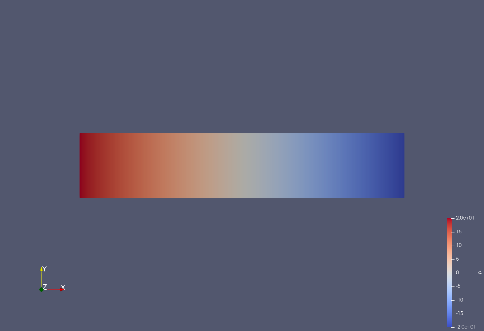
Third we consider mixed boundary conditions on the rectangle [\(0,l\)]\(\times\)[\(0,h\)], where \(l = 5\) its length and \(h = 1\) its height. Non-homogenous Dirichlet conditions are applied on the left side of the rectangle, denoted by \(\Gamma_{inlet}\), non-homogenous Neumann conditions on the right side, \(\Gamma_{outlet}\), and homogenous Dirichlet conditions on the two other sides, \(\Gamma_{wall}\).
The exact solutions are given by:
and
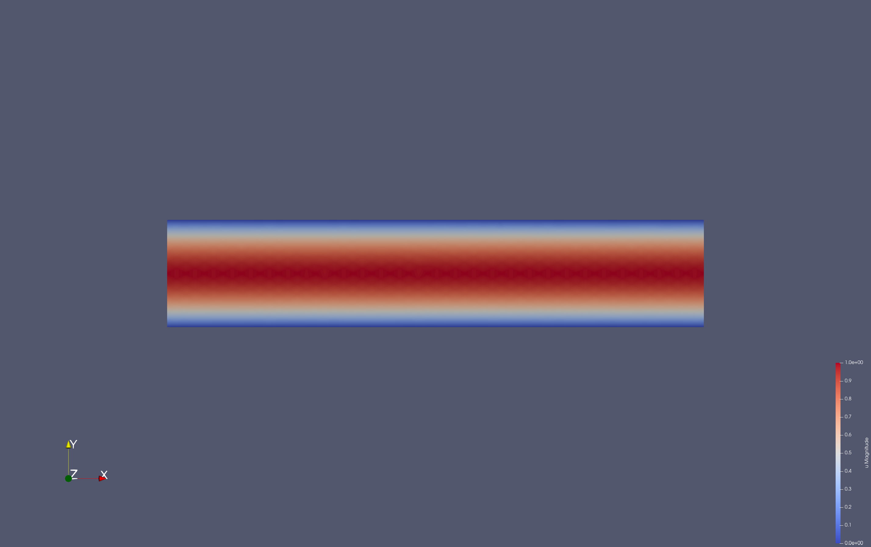
where \(D = \frac{v_{max}}{0.5h(h-0.5h)}\) and \(v_{max} = 1\) the maximal velocity. For the non-homogenous Dirichlet boundary conditions on \(\Gamma_{inlet}\) we use the exact solution of \(u\) and the Neumann conditions on \(\Gamma_{outlet}\) are defined by:
This example is detailed in the Feel++ documentation. By displaying the solution obtained for pressure and velocity, for a mesh size \(h=0.1\), we obtain the same results:
As expected, the errors are equal to \(0\):
\(h\) |
\(\left\Vert u - u_h \right\Vert_{L^2}\) |
\(\left\Vert u - u_h \right\Vert_{H^1}\) |
\(\left\Vert p - p_h \right\Vert_{L^2}\) |
\(0.1\) |
\(2.75061e-15\) |
\(3.62427e-14\) |
\(6.34907e-14\) |
Non-homogeneous Dirichlet boundary conditions 3D
Finally, for the \(3\)D test case, we use the unit cube considering non-homogeneous Dirichlet boundary conditions. The exact solutions are given by:
and
To define the boundary conditions, we use the exact solution of \(u\).
The values of the computed errors are given by the following table:
\(h\) |
\(\left\Vert u - u_h \right\Vert_{L^2}\) |
Order |
\(\left\Vert p - p_h \right\Vert_{L^2} + \left\Vert u - u_h \right\Vert_{H^1}\) |
Order |
\(1\) |
\(0.0242545\) |
\(0.7187319\) |
||
\(\frac{1}{2}\) |
\(0.00615454\) |
\(1.97\) |
\(0.289773\) |
\(1.31\) |
\(\frac{1}{4}\) |
\(0.00197867\) |
\(1.63\) |
\(0.1073367\) |
\(1.43\) |
\(\frac{1}{8}\) |
\(0.000264588\) |
\(2.90\) |
\(0.02356425\) |
\(2.18\) |
\(\frac{1}{16}\) |
\(3.45405e-05\) |
\(2.93\) |
\(0.00551451\) |
\(2.09\) |
The table shows that the orders of convergence are stabilizing around \(3\) and \(2\).