 .pdf
.pdf
Reinforcement learning for the three sphere swimmer with different possible velocities
In this example, we apply reinforcement learning on the three sphere swimmer with more possible actions. Unlike the first study Q-learning_3SS in which the relative velocity was fixed to be 4, here the swimmer can retract or extend each arm with different possible velocities. We aime to check the optimal swimming strategy found by the swimmer using reinforcement learning.
1. Model and Notations
The three sphere swimmer we study here consists of three sphere of raduis \(R=1\) liked by two arms of length \(L=10\). The swimmer can take an action (retracting or extending) with different possible velocities.
Let \(\mathcal{V}\) be the set of the possible velocities given by : \[\mathcal{V}=\bigg\{ v_1, v_2, \dots , v_k\big/ k\geq 2\; and\; 0 <v_i \leq 4\; \forall i\leq k \bigg\}.\]
Retracting or extending an arm with a velocity \(v_i\in\mathcal{V}\) mmeans that the arm is retracted or extended with a length \(\mathcal{\varepsilon_i}\). Since the action is taken in \(T=1s\), we have \(v_i = \varepsilon_i\).
We denote by \(\mathcal{E}=\{\varepsilon_1,\varepsilon_2, \dots ,\varepsilon_k \}\) the set of the possible arms length of retracting or extending with the velocities \(v\in\mathcal{V}\).
1.1. States
The states of the swimmer are characterized by its arms lengths. Here we note a state by a couple \((l_1, l_2)\), where \(l_1\) and \(l_2\) are the lengths of the first and the second arms respectively.
The spaces of states is given explicitly by :
\[\mathcal{S} = \bigg\{(L-\varepsilon_i, L-\varepsilon_j) \big/ \varepsilon_i, \varepsilon_j \in \mathcal{E} \cup \{ 0 \}\bigg\}.\]
It is clear that \(Card(\mathcal{S})= (k+1)^2\). Hence, there are \((k+1)^2\) possible states.
1.2. actions
The swimmer can retract or extend its arms with different velocities (lengths), so we refer to an action by a vector \((a, m, v)\), where :
-
a : refers to the action to perform (either retract or extend)
-
m : refers to which arm the swimmer retracts or extends, here \(m\in\{1,2\}\)
-
v : the velocity of retracting or extending
The space of actions is given as follow :
\[\mathcal{A} = \bigg\{ (a,m,v) \big/ a \in\{retract, extend\}, \; m\in \{1,2\},\; v\in \mathcal{V}\bigg\}.\]
Since \(Card(\mathcal{A})= 4k\), there are in total \(4k\) actions the swimmer can take.
We denote the set of possible actions for a given state \(s\in\mathcal{S}\), by :
\[\mathcal{A_s} = \bigg\{ (a,m,v) \big/ (a,m,v)\in\mathcal{A}\; and\; s_{new}\in\mathcal{S}\bigg\}.\]
For each state, the swimmer can perform only \(2k\) actions.
1.3. Reward
The reward will be the same as defined in Q-learning_3SS.
2. Input parameters
We use the following parameters for the Q-learning algorithm :
Parameter |
Description |
values |
\(\alpha\) |
Learning rate |
1 |
\(\gamma\) |
Discount factor |
0.99 |
\(\epsilon\) |
\(\epsilon\)-greedy parameter |
0.1 |
3. Results
3.1. \(\mathcal{V}=\{2, 4\}\)
Here, we put \(\mathcal{V}=\{2, 4\}\), which means that the swimmer can retract or extend its arms wth two possible velocities (2 and 4).
-
The possible states of the swimmer in this case are given below :
(10, 10), (10, 8), (10, 6), (8, 10), (8, 8), (8, 6), (6, 10), (6, 8), (6, 6)
-
In this case, the swimmer can take 8 actions, but for a given state, there are only 4 possible actions.
Now we show the results of the learning process and the policy found by the swimmer using the Q-learning algorithm.
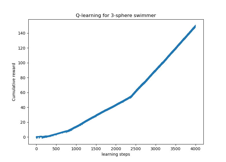
Here, the swimmer has multiple effective swimming strategies. The swimmer initially explore the environement by selecting different actions (different velocities 2 and 4), and finally, after completing 2421 steps of learning, it finds the optimal strategy which is exactly the one proposed by Najafi (Traveling wave with relative velocity \(v=4\)).
3.2. \(\mathcal{V}=\{1, 2, 3, 4\}\)
Now, we add more possible relative velocities and check the optimal policy found by the swimmer. Let \(\mathcal{V}=\{1, 2, 3, 4\}\) be the velicities space.
It is clear that for this case there more states and actions for the swimmer.
-
There are 25 states given as follow :
(10, 10), (10, 9), (10, 8), (10, 7), (10, 6), (9, 10), (9, 9), (9, 8), (9, 7), (9, 6), (8, 10), (8, 9), (8, 8), (8, 7), (8, 6), (7, 10), (7, 9), (7, 8), (7, 7), (7, 6), (6, 10), (6, 9), (6, 8), (6, 7), (6, 6)
-
For this case, there are 16 actions in total, and for each state there 8 possible actions
Now we present the results of the Q-learning algorithm in this case
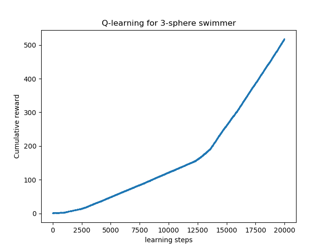
The figure above shows that the swimmer has experienced many policies before it finds the optimal one which corresponds again to Najafi Strokes with the largest relative velocity \(v=4\). Here the swimmer has learnt the optimal strategy after completing 13633 steps of learning.
Here are the states of the swimmer in last twenty one steps of learning :
For N = 19980 the state of the swimmer is  (6, 6)
For N = 19981 the state of the swimmer is  (10, 6)
For N = 19982 the state of the swimmer is  (10, 10)
For N = 19983 the state of the swimmer is  (6, 10)
For N = 19984 the state of the swimmer is  (6, 6)
For N = 19985 the state of the swimmer is  (6, 9)
For N = 19986 the state of the swimmer is  (6, 6)
For N = 19987 the state of the swimmer is  (10, 6)
For N = 19988 the state of the swimmer is  (10, 10)
For N = 19989 the state of the swimmer is  (6, 10)
For N = 19990 the state of the swimmer is  (6, 6)
For N = 19991 the state of the swimmer is  (10, 6)
For N = 19992 the state of the swimmer is  (10, 10)
For N = 19993 the state of the swimmer is  (6, 10)
For N = 19994 the state of the swimmer is  (6, 6)
For N = 19995 the state of the swimmer is  (10, 6)
For N = 19996 the state of the swimmer is  (10, 10)
For N = 19997 the state of the swimmer is  (6, 10)
For N = 19998 the state of the swimmer is  (6, 6)
For N = 19999 the state of the swimmer is  (10, 6)
For N = 20000 the state of the swimmer is  (7, 6)
References on Learning Methods
-
[gbcc_epje_2017] K. Gustavsson, L. Biferale, A. Celani, S. Colabrese Finding Efficient Swimming Strategies in a Three Dimensional Chaotic Flow by Reinforcement Learning Published on Eur. Phys. J. E (December 14, 2017) 10.1140/epje/i2017-11602-9 Download PDF
-
[Q-learning] Tsang, A.C., Tong, P., Nallan, S., Pak, O.S. (2018). Self-learning how to swim at low Reynolds number. arXiv: Fluid Dynamics.Download PDF
References on Swimming
-
[Najafi_2004] Ali Najafi, Ramin Golestanian. Simple swimmer at low Reynolds number: Three linked spheres. 2004. American Physical Society. doi.org/10.1103/PhysRevE.69.062901 linkDownload PDF
-
[nature] Jikeli, J., Alvarez, L., Friedrich, B. et al. Sperm navigation along helical paths in 3D chemoattractant landscapes. Nat Commun 6, 7985 (2015). doi.org/10.1038/ncomms8985 Download PDF
-
[bgp_cemracs_2019] Luca Berti, Laetitia Giraldi, Christophe Prud’Homme. Swimming at Low Reynolds Number. ESAIM: Proceedings and Surveys, EDP Sciences, 2019, pp.1 - 10, doi.org/10.1051/proc/202067004 Download PDF
-
[bcgp_three_spheres_2020] Luca Berti, Vincent Chabannes, Laetitia Giraldi, Christophe Prud’Homme. Modeling and finite element simulation of multi-sphere swimmers. 2020. hal-mines-paristech.archives-ouvertes.fr/ENSMP_CEMEF/hal-03023318v1 Download PDF
-
[gbcc_epje_2017] K. Gustavsson, L. Biferale, A. Celani, S. Colabrese Finding Efficient Swimming Strategies in a Three Dimensional Chaotic Flow by Reinforcement Learning Published on Eur. Phys. J. E (December 14, 2017) 10.1140/epje/i2017-11602-9 Download PDF
-
[purcell_1977] E.M. Purcell. Life at Low Reynolds Number, American Journal of Physics vol 45, p. 3-11 (1977). doi.org/10.1119/1.10903 Download PDF