 .pdf
.pdf
Repulsive force for articulated bodies
- 1. Mathematical formulation
- 2. Test cases
- 2.1. Application : analytical test case to verify implementation
- 2.2. Application : motionless three-sphere swimmer - bottom collision in \(2\)D
- 2.3. Application : tilted motionless three-sphere swimmer - bottom collision in \(2\)D
- 2.4. Application : mobile three-sphere swimmer near boundary in \(2\)D
- References on collision models
1. Mathematical formulation
The purpose of this section is to model the repulsion force for articulated bodies. In particular, we consider the aligned three-sphere swimmer. When the swimmer is placed horizontally in the fluid box without being able to move his rods, then the gravity makes the three spheres of the swimmer fall down with the same velocity, without being subjected to a rotation. However, when considering a tilted swimmer or a swimmer that can retract and extend his rods, one must take into account the torque of gravity and repulsion forces acting on the swimmer. The forces that are applied on the tilted swimmer are visualized by the following figure:
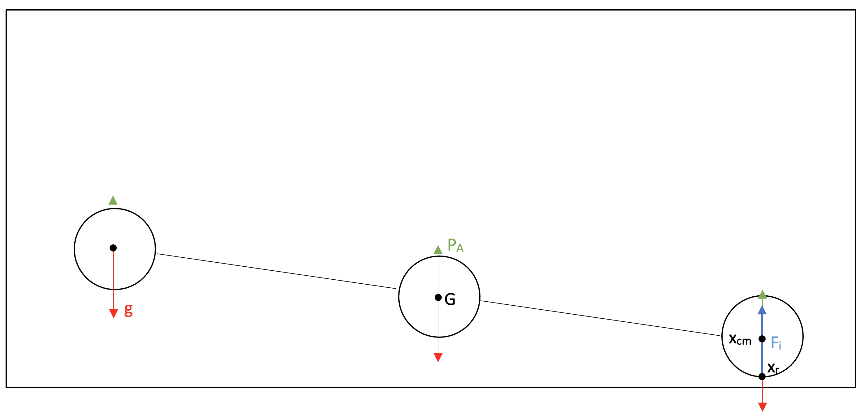
where \(g\) represents the gravity vector, \(P_A\) the buoyancy and \(F_i\) the repulsion force. The center of mass of the swimmer is denoted \(G\), \(x_{cm}\) is the mass center of each sphere and \(x_r\) the point where \(F_i\) is applied on the sphere.
According to the article [Settling_ellipsoid], the terms to be added in Newton’s equation describing the angular velocity of the swimmer are given by:
for each sphere of the swimmer. This Newton’s equation is detailed in section Fluid-body interaction. The algorithm is similar to the one for arbitrary shaped bodies. The insertion of the torque of gravity forces is done in the same way as for collision forces.
2. Test cases
2.1. Application : analytical test case to verify implementation
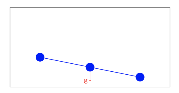
To verify the implementation of this collision algorithm one considers the tilted three-sphere swimmer that is placed close to the domain boundary:
We consider two verifications to validate this case:
-
At first iteration: the coordinate \(y\) of the right sphere is in the interval [\(0,r+\rho\)] and the one of the other spheres are \(> r+\rho\), where \(r\) the radius of the sphere and \(\rho\) the safety zone thickness.
-
At the end of the simulation: all three spheres have their \(y\) coordinate in the interval [\(0,r+\rho\)]. The translation velocity of the three spheres is close to \(0\).
2.2. Application : motionless three-sphere swimmer - bottom collision in \(2\)D
As first test case we consider the collision between the horizontal three-sphere swimmer and the bottom of the fluid box. The swimmer falls under the effect of gravity. We use a motionless swimmer, which does not extend or retract its rods. The parameters are given by:
Name |
Description |
Values |
\(\Omega\) |
Computational domain (box) |
[\(0,6\)] \(\times\) [\(0,2\)] |
\(G\) |
Swimmer center |
(\(3,1\)) |
\(l\) |
Swimmer rod length |
\(1.25\) |
\(\rho_s\) |
Swimmer density |
\(1.25\) |
\(r\) |
Swimmer radius |
\(0.125\) |
\(\rho_f\) |
Fluid density |
\(1\) |
\(\mu\) |
Fluid viscosity |
\(0.1\) |
\(\rho\) |
Safety zone thickness |
\(0.03\) |
\(\epsilon_W\) |
Stiffness parameter |
\(0.00001/2\) |
\(g\) |
Gravity acceleration |
\(\{ 0, -981 \}\) |
\(\Delta t\) |
Simulation time step |
\(10^{-2}\) |
\(h\) |
Simulation mesh size |
\(0.01\) |
We visualize the vertical position and the vertical velocity of the three spheres over time:
As expected, we obtain the same results for the three spheres. One can observe that the position and the vertical velocity become equal to zero.
2.3. Application : tilted motionless three-sphere swimmer - bottom collision in \(2\)D
We consider the collision between the tilted three-sphere swimmer and the bottom of the fluid domain. The swimmer is rotated at an angle \(-\frac{\pi}{24}\) to the horizontal. At the beginning of the simulation, the swimmer’s right sphere is close to the bottom, so the collision force is applied already in the first iteration. The objective of this test is to verify that the torques of the gravity and collision forces are applied. The swimmer is supposed to rotate so that he is horizontally above the bottom.
The parameters used for this test are given by:
Name |
Description |
Values |
\(\Omega\) |
Computational domain (box) |
[\(0,6\)] \(\times\) [\(0,2\)] |
\(G\) |
Swimmer center |
(\(3,0.29\)) |
\(l\) |
Swimmer rod length |
\(1.25\) |
\(\rho_s\) |
Swimmer density |
\(1.25\) |
\(r\) |
Swimmer radius |
\(0.125\) |
\(\rho_f\) |
Fluid density |
\(1\) |
\(\mu\) |
Fluid viscosity |
\(0.01\) |
\(\rho\) |
Safety zone thickness |
\(0.02\) |
\(\epsilon_W\) |
Stiffness parameter |
\(0.00000275\) |
\(g\) |
Gravity acceleration |
\(\{ 0, -981 \}\) |
\(\Delta t\) |
Simulation time step |
\(10^{-2}\) |
\(h\) |
Simulation mesh size |
\(0.01\) |
By showing the vertical position of the three spheres over time, we observe that it gets equal to zero for each:
2.4. Application : mobile three-sphere swimmer near boundary in \(2\)D
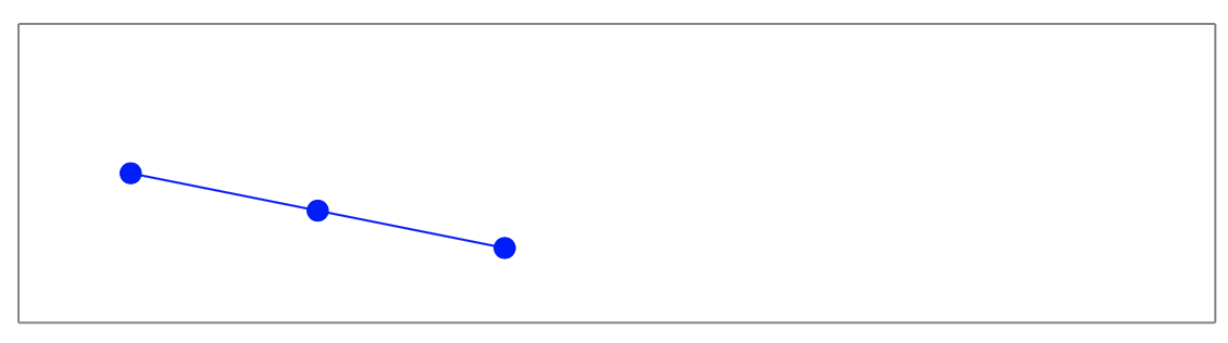
For this last test case we consider a tilted swimmer who is placed in a horizontal channel. The swimmer is initially close to the bottom. The geometry is given by:
The swimmer retracts and extends his arms in order to move. The swimming strategy is defined by:
-
swimmer retracts the left arm
-
swimmer retracts the right arm
-
swimmer extends the left arm
-
swimmer extends the right arm
The purpose of this application is to observe how the swimmer behaves when swimming close to the wall.
The parameters used for this test case are defined by:
Name |
Description |
Values |
\(\Omega\) |
Computational domain (box) |
[\(0,150\)] \(\times\) [\(0,40\)] |
\(G\) |
Swimmer center |
(\(15,10\)) |
\(l\) |
Swimmer rod length |
\(10\) |
\(\rho_s\) |
Swimmer density |
\(0.1\) |
\(r\) |
Swimmer radius |
\(1\) |
\(\rho_f\) |
Fluid density |
\(1\) |
\(\mu\) |
Fluid viscosity |
\(1\) |
\(\rho\) |
Safety zone thickness |
\(0.03\) |
\(\epsilon_W\) |
Stiffness parameter |
\(0.00000005\) |
\(\Delta t\) |
Simulation time step |
\(0.1\) |
\(h\) |
Simulation mesh size |
\(0.3\) |
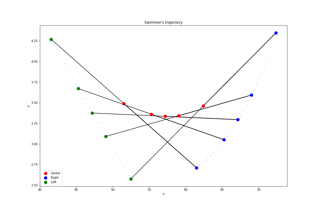
The following graph shows the displacement of the swimmer after each sequence of four swim strokes. At final time, the swimmer has performed \(220\) times this sequence.
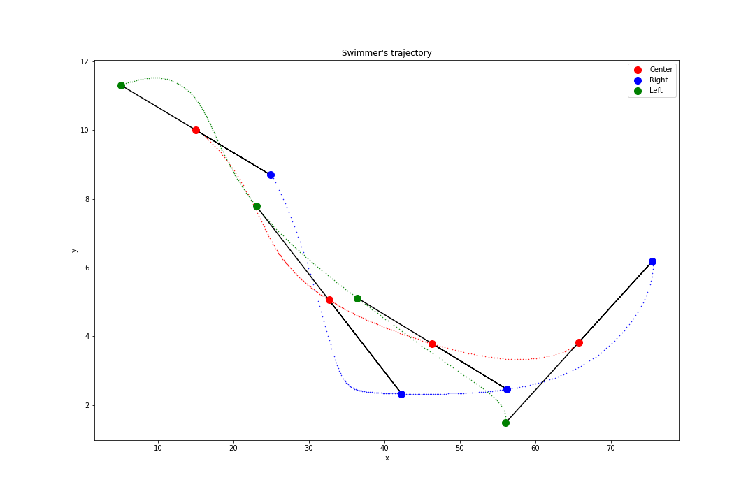
We can observe that at the beginning the swimmer gets closer to the bottom of the channel. Then, when the right sphere is in the lubrication zone, collision forces are applied on it, which then starts to change direction and move upwards. Finally, the swimmer continues to move in this new direction, because of the collision forces that are applied to the left sphere shortly after the rotation
We will observe more in detail the rotation made by the swimmer.
This graph illustrates that the right sphere begins to move away from the boundary when collision forces are applied. The swimmer occupies a horizontal position before his left sphere gets into the lubrication zone. Collision forces are applied that cause the swimmer to continue to move upward.
References on collision models
-
[Glowinski] R. Glowinski, T. W. Pan, T. I. Hesla, D. D. Joseph, and J. Périaux (2000). A Fictitious Domain Approach to the Direct Numerical Simulation of Incompressible Viscous Flow past Moving Rigid Bodies: Application to Particulate Flow. Download PDF
-
[AIP_Advances] K. Usman, K. Walayat, R. Mahmood, et al. (2018). Analysis of solid particles falling down and interacting in a channel with sedimentation using fictitious boundary method. Download PDF
-
[Computers_Fluids] L. Wang, Z.L. Guo, J.C. Mi (2014). Drafting, kissing and tumbling process of two particles with different sizes. Download PDF
-
[Wan_Turek] Decheng Wan and Stefan Turek (2004). Direct Numerical Simulation of Particulate Flow via Multigrid FEM Techniques and the Fictitious Boundary Method. Download PDF
-
[Multiphase_Flow] P. Singh, T.I Hesla, D.D Joseph (2002). Distributed Lagrange multiplier method for particulate flows with collisions.
-
[Settling_ellipsoid] Tsorng-Whay Pan, Roland Glowinski, Giovanni P.Galdi (2001). Direct simulation of the motion of a settling ellipsoid in Newtonian fluid. Download PDF
-
[FMM_1] J.A. Sethian (1996). A fast marching level set method for monotonically advancing fronts.
-
[FMM_2] J.A. Sethian (1996). Level Set Methods and Fast Marching Methods; Evolving Interfaces in Computational Geometry, Fluid Mechanics, Computer Vision and Materials Sciene.
-
[FMM_3] J.A. Sethian. Level Set Methods and Fast Marching Methods.
-
[CollisionModel_DNS] Ramandeep Jain, Silvio Tschisgale, Jochen Fröhlich (2019). A collision model for DNS with ellipsoidal particles in viscous fluid.
-
[DNS_Framework] S.Tschisgale, T.Kempe and J.Fröhlich (2018). A general implicit direct forcing immersed boundary method for rigid particles.
-
[Wu_Shu] J.Wu, C.Shu (2009). Particulate Flow Simulation via a Boundary Condition-Enforced Immersed Boundary-Lattice Boltzmann Scheme.
-
[Stenotic_artery] H.Li, H.Fang, Z.Lin, S.Xu, S.Chen (2004). Lattice Boltzmann simulation on particle suspensions in a two-dimensional symmetric stenotic artery.
-
[Collision_simulations] L.H. Juarez, R. Glowinski, T.W. Pan (2004). Numerical Simulation of Fluid Flow with Moving and Free Boundaries. Download PDF
-
[Collision_ellipticalParticle] Zhenhua Xia, Kevin W. Connington, Saikiran Rapaka, Pengtao Yue, James J. Feng, Shiyi Chen (2008). Flow patterns in the sedimentation of an elliptical particle. Download PDF
-
[Sphere_interaction] S.M. Dash, T.S. Lee (2015). Two spheres sedimentation dynmics in a viscous liquid column.
-
[MMG] www.mmgtools.org/mmg-remesher-try-mmg/mmg-remesher-tutorials/mmg-remesher-mmg2d/implicit-domain-meshing.