Reinforcement learning for the three-sphere swimmer

Here, we apply reinforcement learning algorithm to show how swimmers can self-learn optimal swimming strategies with no prior knowledge and without specifiying any locomotory gaits. The swimmer we treat here is the three sphere swimmer. The self learning will be extended to multiple spheres swimmers (see Q-learning_multispheres).

This approach has already been studied by Alan CH Tsang and other co-workers in their paper [Q-learning].

1. Introduction

We consider the three sphere swimmer that has only one strategy of swimming proposed by Najafi [Najafi_2004]. As we have shown, numericaly, that 2D-three sphere and 3D-three sphere swimmers have similar qualitative net displacements (see 3-spheres-2D), we apply the reinforcement learning on the two dimensional three sphere swimmer.

The double Q-learning algorithm will be also applied to compare its results with Q-learning in term of convergence speed.

2. Reinforcement learning : \(Q\)-learning algorithm

2.1. \(Q\)-Learning

The Q-learning algorithm is a model-free reinforcement learning that seeks to find the best action to take given the current state to maximize the total reward. The experiences results are stored in a \(Q\)-table that is updated over the learning process using the Bellman equation as :

\[Q(s,a) \leftarrow Q(s,a) + \alpha (r + \gamma\cdot\max_{a} Q(s',a) - Q(s,a)),\]

where :

\(\alpha\) : The learning rate
- \(\alpha\) takes values in \([0,1]\)
- When \(\alpha=0\), it means the agent is learning nothing from the previous experiences
- For deterministic environments (where a combinaison [state, action] gives always the same reward), \(\alpha=1\) is the best value that gives optimal convergence for the Q-table
\(\gamma\) : Discount factor
- \(\gamma\) takes values in \([0,1]\)
- It determines the importance of future rewards : When \(\gamma\) is larg (low), the agent is farsighted (shortsighted)
\(r\) : Reward of taking action \(a\) at the state \(s\).

2.2. \(\epsilon\)-greedy scheme

The \(\epsilon\)-greedy scheme is used for more exploration of the environment. In order to discover new states that may not be selected during the exploitation process of Q-learning, we take a random action. To balance between exploration and exploitation, the \(\epsilon\)-greedy algorithm is given as follow :

Select a random action with a probability \(\epsilon\in]0,1[\)
Select the action advised by the Q-table with a probability \(1-\epsilon\)

2.3. \(Q\)-Learning algorithm

The Q-learning algorithm is defined as follow :

Initialize \(s\) and \(Q(s,a)\) to 0
\(\textbf{repeat}\) for each step of learning
- Choose action \(a\) using policy derived from Q (e.g \(\epsilon\)-greedy)
- Take action \(a\), observe \(r\) (reward) and \(s'\) (new state)
- \(Q(s,a) \leftarrow Q(s,a) + \alpha (r + \gamma\cdot\max_{a} Q(s',a) - Q(s,a))\)
- \(s \leftarrow s'\)

2.4. Double \(Q\)-Learning algorithm

The double Q-learning algorithm was proposed to accelerate the convergence rate when Q-learning algorithm performs poorly. Instead of evaluating future action-value with one Q-table, the double Q-learning uses two Q-tables for evaluation.

The algorithm is given as follow :

Initialize \(s\), \(Q^A\) and \(Q^B\)
\(\textbf{repeat}\) for each step of learning
- Choose \(a\), based on \(Q^A(s,\cdot)\) and \(Q^B(s,\cdot)\), observe \(r\), \(s'\)
- Choose (e.g. random) either \(\textit{UPDATE(A)}\) or \(\textit{UPDATE(B)}\)
- \(\textbf{if}\) \(\textit{UPDATE(A)}\) \(\textbf{then}\)
  - Define \(a^* = argmax_{a}Q^A(s',a)\)
  - \(Q^A(s,a) \leftarrow Q^A(s,a) + \alpha (r + \gamma Q^B(s',a^*) - Q^A(s,a))\)
- \(\textbf{else if}\) \(\textit{UPDATE(B)}\) \(\textbf{then}\)
  - Define \(b^* = argmax_{a}Q^B(s',a)\)
  - \(Q^B(s,a) \leftarrow Q^B(s,a) + \alpha (r + \gamma Q^A(s',b^*) - Q^B(s,a))\)
- \(\textbf{end if}\)
- \(s \leftarrow s'\)

3. Self-learn the three sphere swimmer

3.1. States, actions and reward

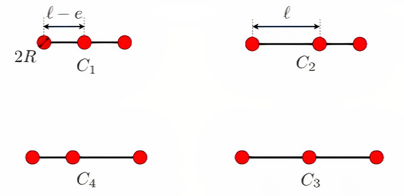
The three sphere swimmer we consider is composed of three spheres of raduis \(R\) linked by two arms of length \(L\). Each arm can be retracted by a length \(\epsilon\).

We fix \(R=1\), \(L=10\) and \(\epsilon = 4R\).

The three sphere swimmer has four states (configurations). The swimmer can switch from one state to another by retrating or extending one of its arms, which results in a net displacement providing a certain reward.

3.1.1. States

The swimmer has four states depending on the length of each arm of the swimmer. The figure below shows these states.

3.1.2. actions

To switch from a state to another, the swimmer has four actions given as follow :

contract left arm
contract right arm
extend left arm
extend right arm

Note that for each state, there are only two possible actions the swimmer can perform.

3.1.3. Reward

We choose the swimmer to be parallel to the \(x\) axis so that the net displacement will only be with respect to the \(x\) axis. In this case, the reward will be the \(x\)-net displacement gained after performing an action in a certain state.

3.2. Interaction with the surrounding fluid meduim

The interaction between the swimmer and the surrounding fluid is simulated using the feelpp fluid toolbox with python. The net displacement of the swimmer will be stored in a \(csv\) file exported by the fluid toolbox.

3.3. Data files

The data files for the three sphere swimmer are available in Github here [Add the link]

add Q-learning file here

3.3.1. Inpute parameters for \(Q\)-learning

For the Q-learning algorithm, we set the following parameters :

Parameter

Description

values

\(\alpha\)

Learning rate

\(\gamma\)

Discount factor

0.95

\(\epsilon\)

\(\epsilon\)-greedy parameter

0.1

4. Results

4.1. Results and remarks

Here, we present the results of Q-learning and double Q-learning algorithms on the three sphere swimmer. The figures below show the cumulative reward in function of learning steps.

learning process of the swimmer and present

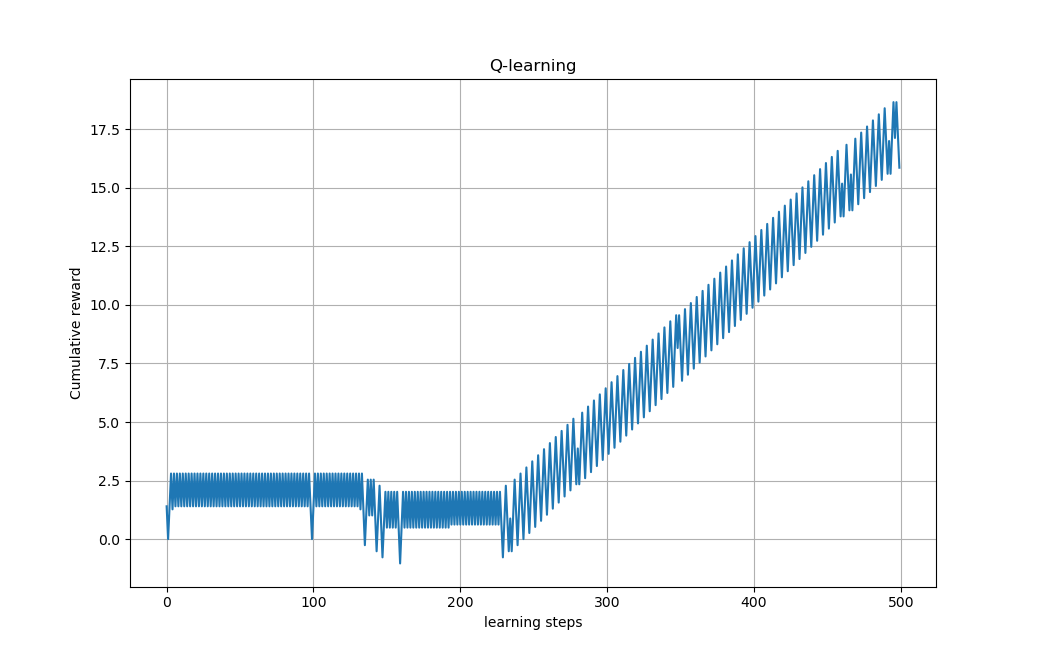
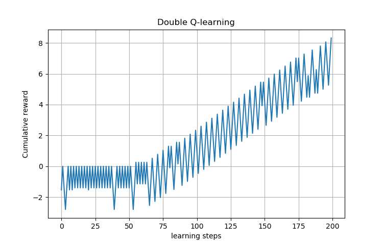
From these figures that show the learning process of the swimmer, we see that the swimmer doesn’t present any net displacement for the first steps of learning. However, it was exploring and trying to accumulate sufficient knowledge about the environment. After enough steps of learning ( \(n\approx 230\) for Q-learning and \(n\approx 65\) for double Q-learning), it finds the effective swimming strategy.

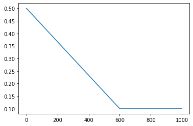
Now, we propose another \(\epsilon\)-greedy scheme as follow : We put \(\epsilon\) as linear function that depends on the learning steps numbers.

\[ \epsilon(N) = \left\{ \begin{array}{ll} \displaystyle{\frac{-0.4}{N_{\epsilon}}N+0.5} & \mbox{if } N\in\{1,2,\cdots ,N_{\epsilon}\} \\ 0.1 & \mbox{if } N\in\{N_{\epsilon},\cdots ,N_{max}\}, \end{array} \right.\]

where \(N_{\epsilon}\leq N_{max}\) is parameter to be chosen and \(N_{max}\) is number of the last learning step.

Wich such function, The probability of taking random actions is higher for the learning steps \(\{1,2,\cdots ,N_{\epsilon}\}\) and this probability is increasing linearly to be 0.1 at \(N_{\epsilon}\) and then it is fixed for the rest of learning steps.

The figure below shows the \(\epsilon\) function with \(N_{max}=1000\) and \(N_{\epsilon}= 600\).

Now

The \(\epsilon\)-greedy scheme is very important for Q-learning, We have generated 100 simulations with the same parameters given above (but \(\epsilon =0\)) for 4000 learning steps. We found that the swimmer has never learnt the traveling wave strategy.

In order to determin the required number of learning steps the swimmer needs to learn the traveling wave, we performed 100 simulations for the two cases :

Test 1 : For \(\epsilon=0.1\) (fixed)
Test 2 : For \(\epsilon\) taking the linear form given above

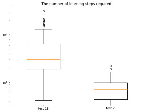
This figure (The vertical scale is logarithmic in base 10) shows that in the second test, the swimmer finds the optimal policy quickly compared to the first test in which we fixe \(\epsilon = 0.1\).

5. Conclusion

Here, using a simple reinforcement learning algorithm we show that the three sphere swimmer can self-learn the swimming strategy with no prior knowledge about the scallop theorem or any locomotory specification. More complexe models such as swimmers with incresed number of spheres were studied in Q-learning_multispheres

References on Learning Methods

[gbcc_epje_2017] K. Gustavsson, L. Biferale, A. Celani, S. Colabrese Finding Efficient Swimming Strategies in a Three Dimensional Chaotic Flow by Reinforcement Learning Published on Eur. Phys. J. E (December 14, 2017) 10.1140/epje/i2017-11602-9 Download PDF
[Q-learning] Tsang, A.C., Tong, P., Nallan, S., Pak, O.S. (2018). Self-learning how to swim at low Reynolds number. arXiv: Fluid Dynamics.Download PDF

References on Swimming

[Najafi_2004] Ali Najafi, Ramin Golestanian. Simple swimmer at low Reynolds number: Three linked spheres. 2004. American Physical Society. doi.org/10.1103/PhysRevE.69.062901 linkDownload PDF
[nature] Jikeli, J., Alvarez, L., Friedrich, B. et al. Sperm navigation along helical paths in 3D chemoattractant landscapes. Nat Commun 6, 7985 (2015). doi.org/10.1038/ncomms8985 Download PDF
[bgp_cemracs_2019] Luca Berti, Laetitia Giraldi, Christophe Prud’Homme. Swimming at Low Reynolds Number. ESAIM: Proceedings and Surveys, EDP Sciences, 2019, pp.1 - 10, doi.org/10.1051/proc/202067004 Download PDF
[bcgp_three_spheres_2020] Luca Berti, Vincent Chabannes, Laetitia Giraldi, Christophe Prud’Homme. Modeling and finite element simulation of multi-sphere swimmers. 2020. hal-mines-paristech.archives-ouvertes.fr/ENSMP_CEMEF/hal-03023318v1 Download PDF
[gbcc_epje_2017] K. Gustavsson, L. Biferale, A. Celani, S. Colabrese Finding Efficient Swimming Strategies in a Three Dimensional Chaotic Flow by Reinforcement Learning Published on Eur. Phys. J. E (December 14, 2017) 10.1140/epje/i2017-11602-9 Download PDF
[purcell_1977] E.M. Purcell. Life at Low Reynolds Number, American Journal of Physics vol 45, p. 3-11 (1977). doi.org/10.1119/1.10903 Download PDF