Performance

As reconstruction of mesh from a point cloud is an hard operation to perform, the complexity of most algorithm able have a complexity of O(n³), The main objective of the KSR algorithm is to enhance perfomance by reducing the number of tiny cells responsible for small artifacts and more execution time and memory usage

As we look through the user manual of KSR package footnote:https://cgal.geometryfactory.com/CGAL/doc/master/Kinetic_surface_reconstruction/index.html[KSR] we have access to some test and the time requiered for each.

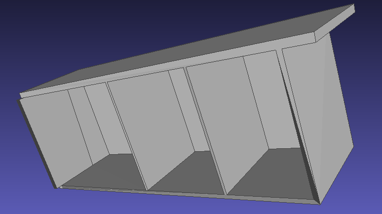
Exemple of Ksr output from CGAL,from left to right input,output,superposition ,from up to down :meeting room,Full thing,Hilbert cube user manual

images::KSREXEMPLE.png[width=300]

With the following execution time :

Table 1. Execution times from CGAL user manual
Mesh	meeting room	Full thing	Hilbert cube
Kinetic shape detection	37.1s	8.6s	0.6s
Kinetic space partition	93.4s	238.8s	10.5s
Total Time	131.1s	248.2s	11.1s

There are some other operations that take time but are negligible compared to detection and partition. Since our focus is primarily on building meshes, we will compare our performance results with the meeting room execution time provided in the KSR user manual.

Initially, during our project earlier in the year we attempted to use the KSR algorithm directly with STL file data. and even if mesh like Three zones are really simple, the algorithme would not work. So we used software like cloodcompare to generate point cloud and as an outcome it would take some hours to generate a mesh with KSR algorithm with our personal computer. After that during the intership I mainly try everything using the super-computer Gaya.After working a bit to generate a good point cloud with good normals we could reduce the execution time by a lot

Figure 1. Result from the start of internship

For this result the shape detection took 124s and the kinetic space partion 0.2s.When compare to the size and the complexity of the meeting room mesh, it kinda disapointing. But after this we decided to implemente the grid simplify function to unified the mesh.And so we could had way better result like

Figure 2. Result after grid simplify

Execution time : 1.6s for shape detection and 1.1 for space partition

When using the KSR algorithm, two primary parameters significantly influence execution time: maximum.distance and min.region.size. Increasing or reducing each value would change the number and shape of detected shape. Adjusting these parameters can either speed up or slow down the process, depending on the desired level of detail and accuracy.

Table 2. Execution time with our workflow on Three zones
Parameters	default : min.region.size=3847 ,maximum.distance=0.44	min.region.size=2000,maximum.distance=0.08	min.region.size=500,maximum.distance=0.08	min.region.size=100,maximum.distance=0.08
Shape detection	7.97s	8.18s	5.76s	1.62s
Kinetic space partition	0.22s	0.22s	0.36s	1.35s
total execution	8.2s	8.41s	6.13s	2.98s

We can do the same for ACjasmin

Table 3. Execution time on ACJasmin
Parameters	default : min.region.size=7512,maximum.distance=0.49	min.region.size=3000,maximum.distance=0.08	min.region.size=2000,maximum.distance=0.08	min.region.size=1200,maximum.distance=0.06
Shape detection	407s	58s	39.8s	31.5s
Kinetic space partition	0.4s	0.8s	0.7s	0.9s
Total execution	407.5s	58.8s	40s	32.5s

We can observe a significant reduction in execution time when we adjust the values of the parameters. The difference in output will be discussed in the section Result. This indicates that the execution time highly depends on selecting the most appropriate parameters for the desired outcome and the input mesh.

Additionally, our main includes other functions, such as the point cloud generator and exporter, which can impact the overall execution time. One of the significant issue when using the KSR algorithm is the unpredictability of the chosen parameters effectiveness.Moreover, improper parameter selection can lead to execution failures, such as segmentation faults.

Next Conclusion