Monte Carlo Method

Monte Carlo methods are a set of statistical simulation techniques used to estimate numerical results based on random sampling. Let’s start with an example:

1. Example Estimating the Value of $\pi$

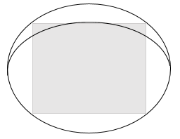
We want to estimate the value of $\pi$ using the Monte Carlo method. The idea is to calculate $\pi$ by comparing the area of a circle inscribed in a square with the total area of the square.

We know that area of square is $A_s = s^2$ and cercle is $A_c = \pi \frac{s}{2} $, where $s$ is the side length of the square.

Throw Random Points:

Generate a large number of random points inside the square. For example, let’s generate $N$ points.
For each point, check if it falls inside the circle or not.

Count the Points Inside the Circle:

Count the number of points that fall inside the circle. Let’s say this number is $M$

Estimate $\pi$:

The fraction of points that fall inside the circle relative to the total number of points is an estimate of the area of the circle divided by the area of the square.
Therefore, the estimate of $\pi$ is given by the formula:

\[ \pi ≈ A_s * \frac{M}{N}\]

Here, $A_s$ is square area, and we want to obtain the area of the circle.

Numerical Example:

Define the Square and the Circle:
Square: side length $2$, area $= 4$
Circle: radius $1$, area $= \pi$
Generate Points:
Suppose we generate $10000$ random points in the square.
Count Points Inside the Circle:
After checking, suppose $7850$ points fall inside the circle.
Calculate $\pi$:
The fraction of points inside the circle is $\frac{7850} {10000} = 0.785$.
Estimate of $\pi$:

\[ \pi ≈ 4 * 0.785 = 3.14\]

This example shows how the Monte Carlo method can be used to estimate $\pi$ based on random sampling and geometric principles. The more points we throw, the more accurate our estimate will be.

2. Calculating View Factors

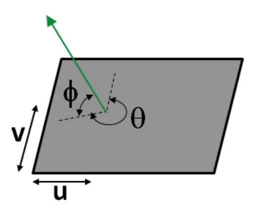
To calculate a view factor, our Monte Carlo simulation should represent the perspective from one surface over the area that the surface can see for instance, a flat plate surface can see an entire hemisphere

Figure 1. Flat plate surface

Our integration scheme will require sampling across the entire area of the plate (u, v), as well as all angles (θ, φ). For each ray, four random numbers are needed.

Figure 2. Random numbers

Figure 3. Consider the following geometry all surfaces are opaque

Let’s shoot 1000 rays from Surface 1;

200 rays hit Surface 2;

150 rays hit Surface 3;

80 rays hit Surface 4;

The rest escape to space

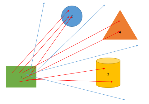
Figure 4. Consider the following geometry all surfaces are opaque

The view factor between Surface 1 and the others is:

$ F_{12} = 200/1000 = 0.200 $

$ F_{13} = 150/1000=0.150 $

$ F_{14} = 80/1000 = 0.080 $

$ F_{1SPACE} = 570/1000 = 0.570 $

We also see that:

$ F_{12} + F_{13} + F_{14} + F_{1SPACE} = 0.200 + 0.150 + 0.080 + 0.580 = 1.000 $

In all cases, view factors must sum to unity

Consider two parallel unit plates separated by one unit, we’ll apply the Monte Carlo method to calculate the view factor between these two surfaces

Figure 5. 20 rays

Figure 6. 100 rays

Figure 7. 500 rays

Figure 8. 1000 rays

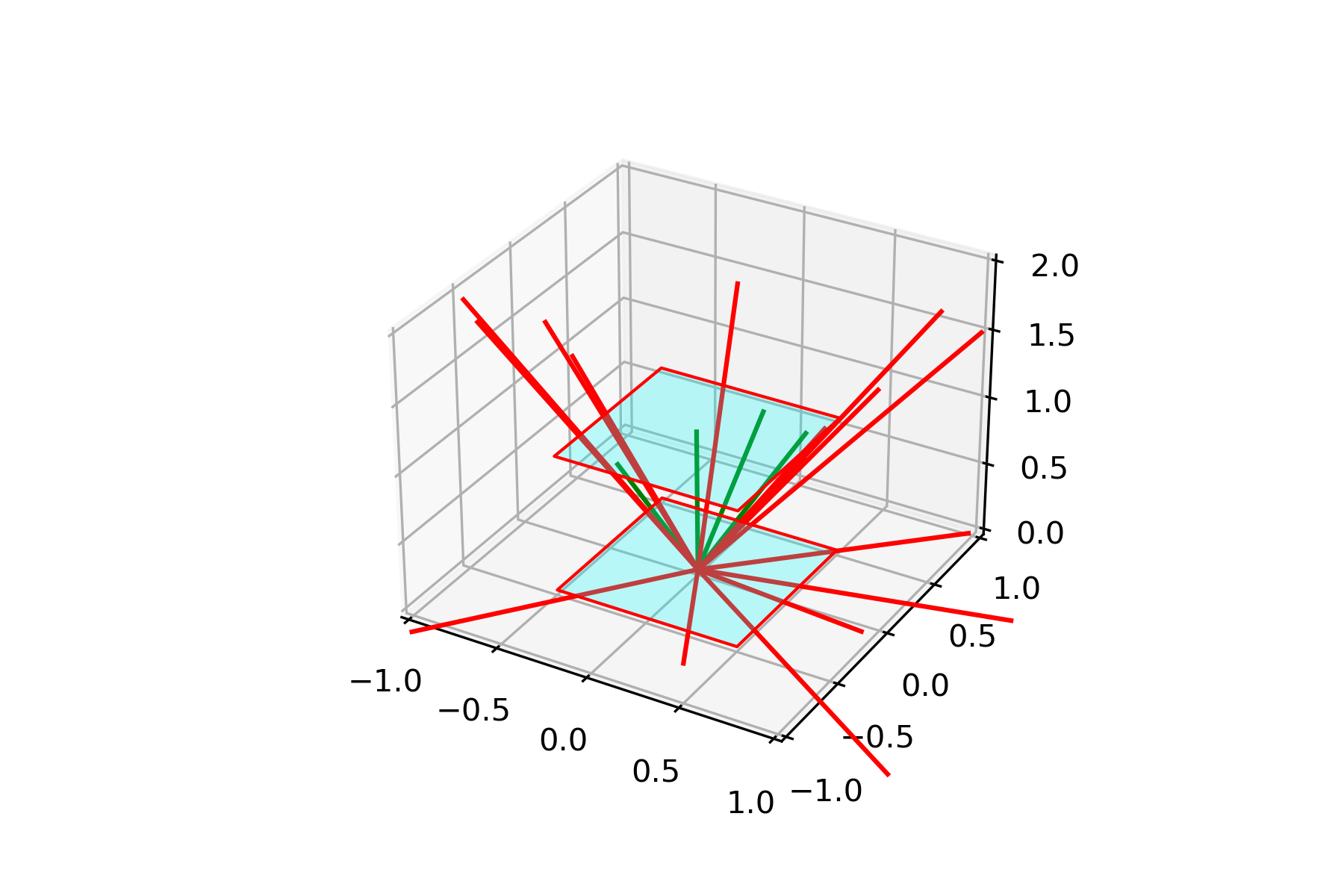
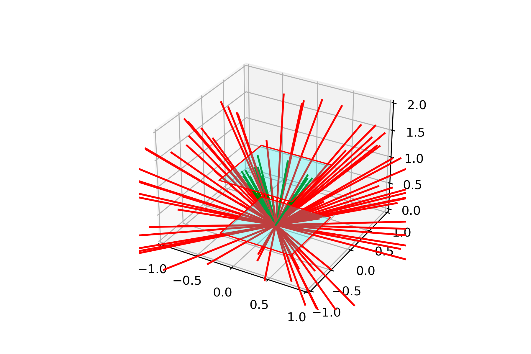
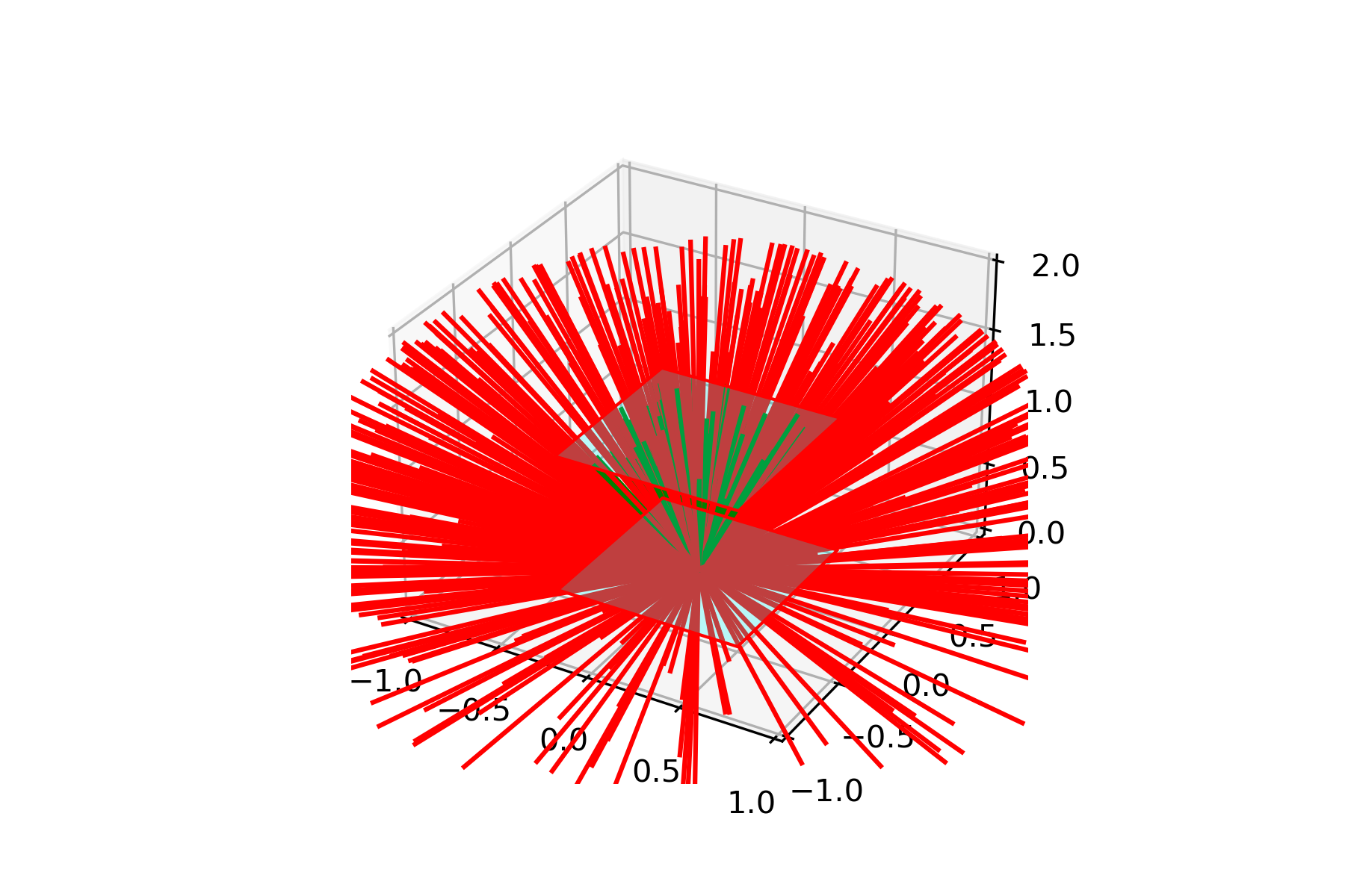
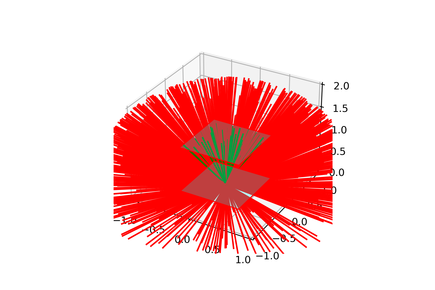
In this part of the code, we generate direction sampling: The getRandomDirection function produces random directions uniformly distributed over a sphere or a circle, depending on the dimension (2D or 3D). It adjusts the direction based on the surface normal to ensure that the directions are correctly oriented

 void getRandomDirection(std::vector<double> &random_direction, std::mt19937 & M_gen, std::mt19937 & M_gen2,Eigen::VectorXd normal)
 {
 std::cout << "normal " << normal << std::endl;
 std::cout << std::flush;
 printf("normal %f %f %f\n", normal[0], normal[1], normal[2]);
 std::uniform_real_distribution<double> xi2(0,1);
 std::uniform_real_distribution<double> xi1(0,1);
 int size = random_direction.size();
 Eigen::VectorXd z_axis(size), crossProd1(size), crossProd2(size),crossProd3(size), direction(size);
 Eigen::MatrixXd matrix1(size,size), matrix2(size,size);
 if(random_direction.size()==3)
 {
     z_axis << 0, 0, 1;
     double phi = 2.*M_PI*xi1(M_gen);
     double theta = math::asin(math::sqrt( xi2(M_gen2)));
     random_direction[0]=math::sin(theta)*math::cos(phi);
     random_direction[1]=math::sin(theta)*math::sin(phi);
     random_direction[2]=math::cos(theta)
     if( math::abs(normal.dot(z_axis)) < 1)  // if the normal is not aligned with z-axis,
                                             // rotate random_direction according to the rotation bringing normal to z-axis
     {
         direction << random_direction[0],random_direction[1],random_direction[2];
         crossProd1 = ((z_axis).head<3>()).cross((normal).head<3>());
         crossProd2 = ((crossProd1).head<3>()).cross((z_axis).head<3>());
         crossProd3 = ((crossProd1).head<3>()).cross((normal).head<3>());
         matrix1.col(0) = z_axis;
         matrix1.col(1) = crossProd2;
         matrix1.col(2) = crossProd1;
         matrix2.row(0) = normal;
         matrix2.row(1) = crossProd3;
         matrix2.row(2) = crossProd1;
         direction = matrix1 * (matrix2 * direction);
         random_direction.resize(direction.size());
         Eigen::VectorXd::Map(&random_direction[0], direction.size()) = direction;
     }
 }
 else if (random_direction.size()==2)
 {
     double phi = M_PI*xi1(M_gen);
     random_direction[0]=math::cos(phi);
     random_direction[1]=math::sin(phi);
  }
 else
 {
     throw std::logic_error( "Wrong dimension " + std::to_string(random_direction.size()) + " for the random direction" );
 }
 //return random_direction;
}

and we use these random variables for ray tracing:

std::random_device M_rd;  // Will be used to obtain a seed for the random number engine
std::random_device M_rd2;  // Will be used to obtain a seed for the random number engine
std::mt19937 M_gen; // Standard mersenne_twister_engine seeded with rd()
std::mt19937 M_gen2; // Standard mersenne_twister_engine seeded with rd2()

We generate these rays using the following code: In the computeViewFactor_bvh function, rays are emitted from random points on mesh elements in random directions, and intersections with other elements are determined using the BVH. This process involves multiple rays per element, which is characteristic of the Monte Carlo method.

 auto rays_from_element = [&](int n_rays_thread){
 Eigen::VectorXd row_vf_matrix(M_view_factor_row.size());
 row_vf_matrix.setZero();
 for(int i=0;i<n_rays_thread;i++)
 {
     // Generate a random point and direction
     auto random_origin = get_random_point(el.second.vertices());
     Eigen::VectorXd rand_dir(dim);
     getRandomDirection(random_direction, M_gen, M_gen2, element_normal);
     // Create ray and check for intersections
     bvh_ray_type ray(origin, rand_dir, 1e-8);
     auto rayIntersectionResult = M_bvh_tree->intersect(_ray=ray);
     // Process intersections...
 }
 return row_vf_matrix;
};

back to main page