View Factors in Radiative Computations

1. Heat Transfer and View Factors

Heat transfer can occur by the three previous methods. Thermal conduction is induced by a temperature gradient between two entities in physical contact.

Figure 1. Net radiation heat exchange between two surfaces

Fourier’s law formulates the heat flux density q as the product of thermal conductivity k by the temperature gradient -∇T, which can be written as follows:

\[ q = -k \nabla T \tag{1} \]

The rate of conductive heat transfer can be expressed as:

\[ \phi_{1−2} = −kA(T_2 − T_1)/d \tag{2} \]

where A denotes the cross-sectional surface area and d denotes the distance between the ends (such as material thickness).

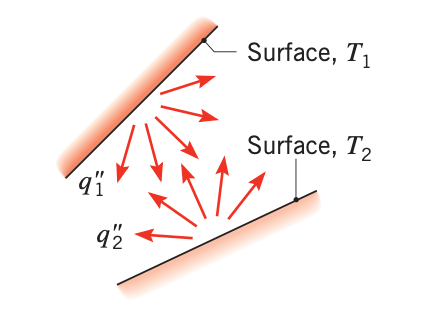
Radiative heat transfer between two surfaces (noted 1 and 2) is the radiation leaving the first surface for the other minus the one arriving from the second surface. The Stefan-Boltzmann law yields:

\[\phi_{1−2} = σA_1F_{1−2}(T_1^4 − T_2^4) \tag{3} \]

where σ denotes the Stefan-Boltzmann constant, A_{1} denotes the area of the first surface and \(F_{1-2}\) denotes the view factor from 1 to 2 (unitless).

Radiosity problems and radiative thermal simulations are governed by a geometric quantity referred to as the view factor, also referenced as shape factors, form factors, configuration factors or angle factors (see equation (3)). Given two surfaces 1 and 2, the view factor \(F_{1-2}\) measures the proportion of the radiation which leaves 1 and strikes 2. More specifically, the view factor quantity measures the fraction of the heat flux radiated by an isothermal surface with isotropic emission received by another surface in a non-participatory environment (no emission, absorption or diffusion). This value depends only on the geometry of the environment. Such a proportion is lower in the presence of obstacles that reduce radiation or incur shadows on 2.

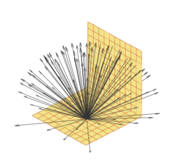
The view factor, \(F_{ij}\), between two small areas, \(A_{i}\) and \(A_{j}\), is the fraction of radiation emitted by area A_{i} that is intercepted by area \(A_{j}\). Essentially, \(F_{ij}\) measures the direct visibility between \(A_{i}\) and \(A_{j}\), influenced by their orientation and the distance separating them. Within a uniform hemispherical light transport or heat transfer model, assuming no obstructions, the exact value of \(F_{ij}\) for two infinitesimal surfaces, \(dA_{i}\) and \(dA_{j}\), is determined by the view factor \(dF_{ij}\) as follows:

\[dF_{ij} = \frac{\cos\Theta_i \cos\Theta_j }{\pi R_{ij}^2} dA_j \tag{4} \]

where \(\Theta_{i}\) and \(\Theta_{j}\) are the angles between the unit normals to the areas and the line \(R_{ij}\) connecting the two areas.

If the two areas are finite, then the view factor is given by:

\[F_{ij} = \frac{1}{A_i} \int_{A_i} \int_{A_j} \frac{\cos\Theta_i \cos\Theta_j }{\pi R_{ij}^2} dA_i dA_j \tag{5} \]

Figure 2. Uniform hemispherical model

Figure 3. Configuration of two surface elements

2. View factor properties:

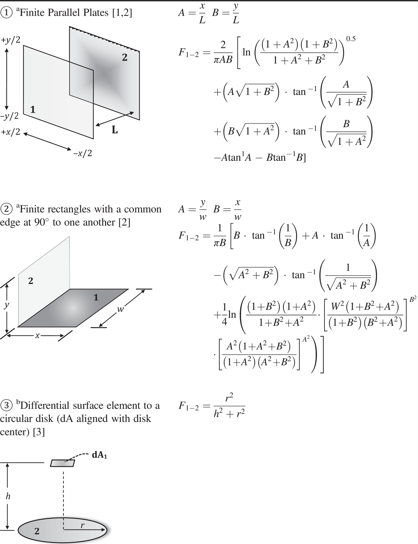
\[ \text{Summation:} \quad \sum_{j=1}^{n} F_{Si \rightarrow Sj} = 1 \] \[ \text{Superposition:} \quad F_{1 \rightarrow (2,3)} = F_{1 \rightarrow 2} + F_{1 \rightarrow 3} \] \[ \text{Reciprocity:} \quad A_1 F_{1 \rightarrow 2} = A_2 F_{2 \rightarrow 1} \] \[ \text{Planar or convex surface:} \quad F_{1 \rightarrow 1} = 0 \] \[ \text{Concave surface:} \quad F_{1 \rightarrow 1} \neq 0 \]

3. Computing View Factors

While view factors can be computed in closed form for certain classes of canonical surfaces without obstacles, general free-form surfaces require calculating complex integrals with quadrature schemes. Until recently, the quadruple integrals were computed by hand for the most common configurations in order to have an exact and rapid evaluation, easy to implement for small computers. In this image we can see somme methods to computing view factors by diffrent geometric

Figure 4. Some value of view factors for diffrent surfaces

4. Example

Figure 5. Half-sphere

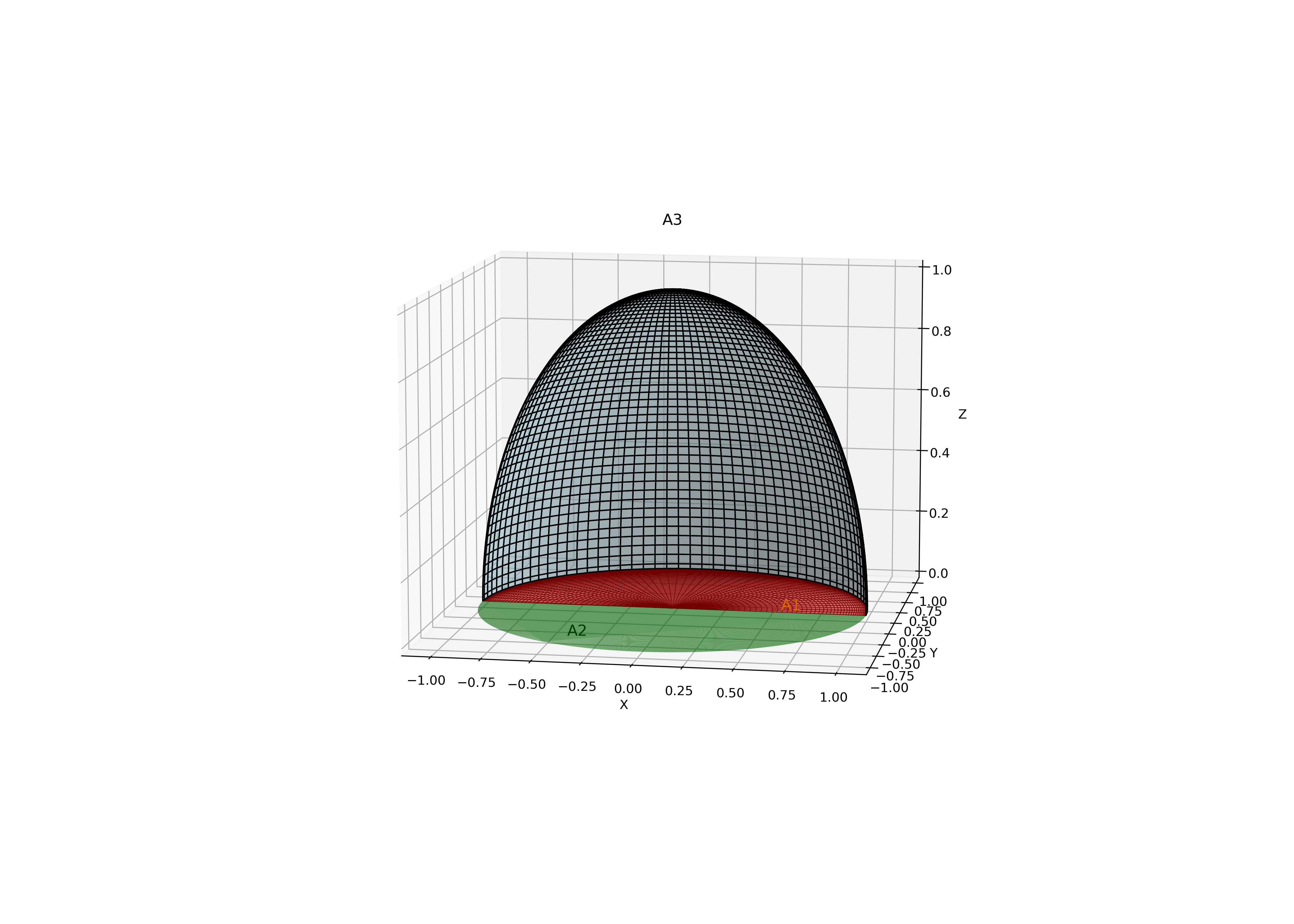
We take an empty half-sphere with its base divided into two. This means we have three faces: \(A_1, A_2\), and \(A_3\). In this example, the dimension is \(n^2 = 9\) because \(n = 3\).

So we have this matrix:

\[\begin{equation} \begin{pmatrix} F_{11} & F_{12} & F_{13} \\ F_{21} & F_{22} & F_{23} \\ F_{31} & F_{32} & F_{33} \\ \end{pmatrix} \end{equation}\]

To calculate the value of each element, we start by considering the properties of view factors. Since surfaces \(A_1\) and \(A_2\) are planar, we have \(F_{11} = F_{22} = 0\). Also, because the planes \(A_1\) and \(A_2\) are in contact, \(F_{12} = F_{21} = 0\).

We know that \(F_{11} + F_{12} + F_{13} = 1\), which means \(F_{13} = 1\). The same applies to \(F_{23} = 1\).

By reciprocity, we have:

\[F_{31} = \frac{A_1}{A_3} F_{13}\]

and similarly:

\[F_{32} = \frac{A_2}{A_3} F_{23}\]

The last element can be concluded by the sum of these elements:

\[F_{31} + F_{32} + F_{33} = 1\]

so:

\[F_{33} = 1 - \frac{A_1 + A_2}{A_3}\]

Finally, the matrix of view factors is :

\[\begin{equation} \begin{pmatrix} 0 & 0 & 1 \\ 0 & 0 & 1 \\ \frac{A_1}{A_3} & \frac{A_2}{A_3} & 1 - \frac{A_1 + A_2}{A_3} \\ \end{pmatrix} \end{equation}\]

back to main page